


Create a Differential Interferogram
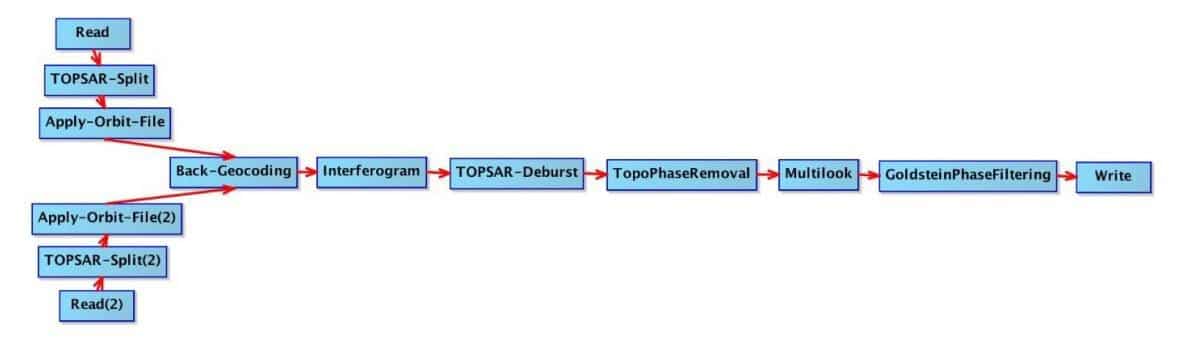
Detailed information on completing this procedure is covered in the ASF Interferogram Generation data recipe. The diagram shown in Figure 3 and the list of the processing steps, which reference the menu options leading to the tool for each step, give an overview of the steps required to generate a wrapped interferogram.
a) Coregistration
Radar > Coregistration > S1 TOPS Coregistration > S-1 TOPS Coregistration
b) Create Interferogram
Radar > Interferometric > Products > Interferogram Formation
c) Deburst
Radar > Sentinel-1 TOPS > S-1 Deburst
d) Topographic Phase Removal
Radar > Interferometric > Products > Topographic Phase Removal
e) Multilook
Radar > Multilooking
f) Goldstein Phase Filtering
Radar > Interferometric > Filtering > Goldstein Phase Filtering
Note: This process chain does not include a Geocoding step. This will be done near the end of this recipe, once the deformation map is generated.
If you geocoded the Unwrapped Interferogram in the previous recipe, make sure to use the product from the step prior to geocoding (not tagged with a _TC) for the next step.
Unwrap the Interferogram
Detailed information on completing this procedure is covered in the ASF Phase Unwrapping data recipe. A brief overview of the steps in that process is presented below.
a) Snaphu Export
Radar > Interferometric > Unwrapping > Snaphu Export
b) Snaphu Unwrapping in a Linux command line
c) Snaphu Import
Radar > Interferometric > Unwrapping > Snaphu Import
Note: This process chain again does not include a Geocoding step. This will be done near the end of this recipe, once the deformation map is generated.
If you Geocoded the Unwrapped Interferogram in the previous recipe, make sure to use the product from the step prior to geocoding (not tagged with a _TC) for this next step.
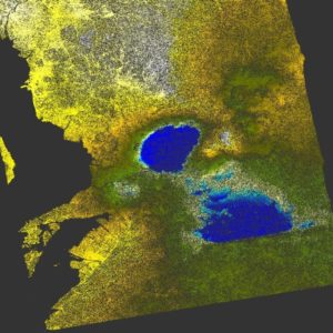
At this point, you should have an unwrapped interferogram (Figure 4) loaded into the Sentinel-1 Toolbox (S1TBX). This recipe will resume from here.

This is computed using the following equation: 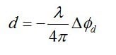
Where λ is Sentinel-1’s C-band SAR wavelength and ![]() is the unwrapped phase difference between the two SLC images.
is the unwrapped phase difference between the two SLC images.
1. Select the imported and unwrapped interferogram in the Product Explorer window in S1TBX. If the Product Explorer window is not open, select Tool Windows from the View menu and select Product Explorer to open it.
2. Navigate to Radar > Interferometric > Products > Phase to Displacement.

3. In the Phase to Displacement window, specify the output folder and the target product name.
- The products will automatically be appended with the suffix “_dsp” if you choose the default name.
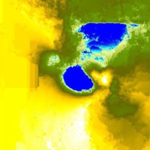
- There will be no options available in the Processing Parameters tab. Click <Run> and allow the image to be processed. The new product, appearing in the Product Explorer window, will have a single band (Figure 5).


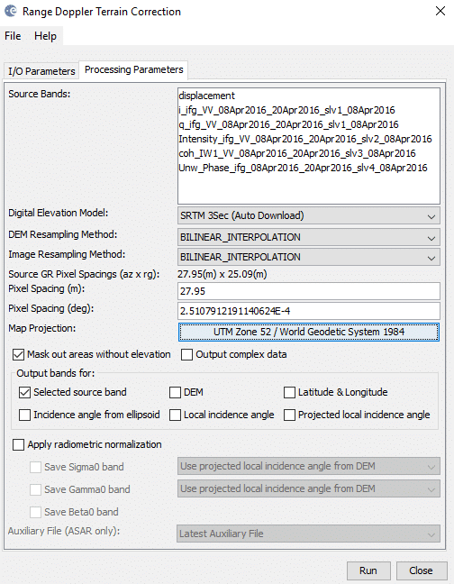
3. In the I/O Parameters tab in the Range-Doppler Terrain Correction window, specify the target product name and the output folder. The products will automatically be appended with the suffix “_TC” if you choose the default name.
4. In the Processing Parameters tab (Figure 6), set the Map Projection by clicking on the Map Projection option. In the window that appears, select UTM Zone / WGS 84 (Automatic) from the Projection options. This will apply the appropriate UTM zone for the image location (best for GIS).
NOTE: If you want to export KMZ files for use in Google Earth as your primary product, leave the Map Projection as WGS84(DD).
Also note that the SRTM, which is the default DEM, does not have coverage beyond 60 degrees north and south. If your granules are located above 60 degrees north, you will need to select a DEM that covers that area, such as ACE30.
5. Leave the rest of the parameters as default and click <Run>.
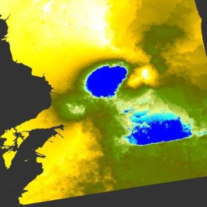
6. When processing is complete, close the Correction window and view the product (Figure 7) by double-clicking the band.
Step 4: Mask Out Areas of Low Coherence
1. In the Product Explorer, right-click the terrain corrected displacement map stack created in Step 3 and select Band Maths.
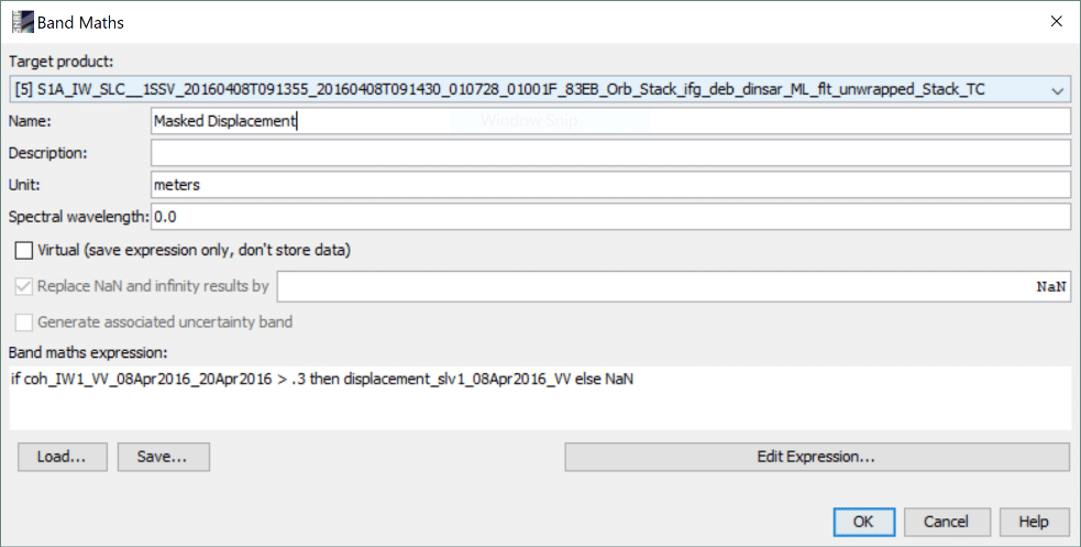
2. In the Band Maths window (Figure 8), set the Name to something appropriate, such as Masked Displacement.
3. Copy and paste the following expression into the Band maths expression field:
if coh_IW1_VV_20Apr2016_08Apr2016 > .3 then displacement_slv1_20Apr2016_VV else NaN
4. Click <OK>. A new band will appear in the product’s Bands folder, and the image will appear in the view area (Figure 9).
Step 5: Update Color Scheme
1. Ensure that the masked displacement band is open and displayed in the view area.
2. Click on the Colour Manipulation tab in the lower left corner of S1TBX to view the Color Manipulation window (Figure 10). If the Colour Manipulation window is not open, select Tool Windows from the View menu and select Colour Manipulation to open it.
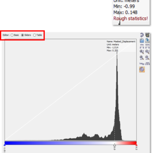
3. Click the circle by Sliders in the top left corner of the window if necessary to open the Sliders Editor view (see Figure 10).
4. Click on the Rough Statistics! text in the top right of the graph pane and click <Yes> in order to calculate accurate displacement statistics for the color scheme.
5. Select the Basic view in the top left region of the tab. Select great_circle from the colour ramp options, and click the Range from Data button.
6. Return to the Sliders view. Right-click the triangle slider on the far left of the color scale and select Remove Slider.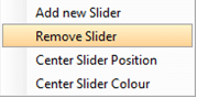
There are two sliders almost on top of each other on the left side of the color ramp, and this will remove the extra one.
7. Select the Table view. There should be three entries with data values listed for each color: blue, white and red. If the first color is black, click on the colour patch and change it to blue. Double-click on the value next to white and change it to 0. Press Enter to apply the change. If there are more than three values, return to the Sliders view and remove the extra sliders.
The resulting displacement map (Figure 11) displays the change in the distance along the line-of-sight from the sensor to the earth’s surface.
If the image acquired on the earlier date was used as the master in this process, positive values (displayed in red on this color scale) will indicate areas that are closer to the sensor in the later acquisition than they were in the earlier acquisition. This could indicate either vertical uplift or horizontal displacement in the direction towards the sensor, but is most often a combination of both.
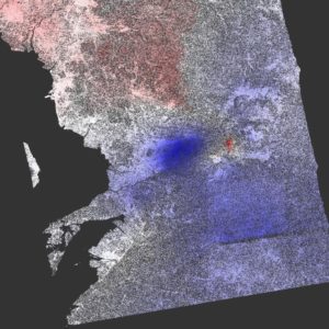
Negative values (displayed in blue on this color scale) indicate either subsidence or horizontal displacement in the direction away from the sensor, but again is most often a combination of both. Areas displayed in white indicate regions without change.
Step 6: Export as GeoTIFF
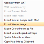 1. Right-click in the view area on your masked and re-colored displacement map. Select Export View as Image, and save the file.
2. In the upper right-hand side of the new window (Figure 12), select Full Screen.
3. Next to Files of type select GeoTIFF.
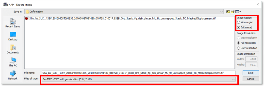
4. Click <Save>.
View in Google Earth (OPTIONAL)
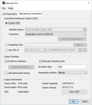
To export to KMZ format, the Masked Displacement band must be in a Geographic Coordinate System (lat/lon). If you output to a UTM projection during Terrain Correction in Step 3, you will need to reproject the output to WGS 84 (Figure 13). Alternatively, you can rerun Step 3 projecting to WGS 84 instead of UTM, then repeat Steps 4 and 5.
Subset Bands (OPTIONAL)
It takes a while to reproject an entire stack, so you may wish to create a subset with only the bands required for the Masked Displacement output first before reprojecting.
1. Select the final product (which includes the Masked Displacement band), and from the menu bar, navigate to Raster > Subset.
2. Select the Band Subset tab and select only the Masked Displacement, coh and displacement bands. Note that if you only select the Masked Displacement band, S1TBX pops up a window prompting you to select the reference datasets (coherence and displacement) as well.
3. Click <OK> to generate the subset. The output will be prefixed with subset and added to the Product Explorer.
Reproject Subset Bands
Select the subset product (or the full product including the Masked Displacement if you want to reproject all of the bands) in the Product Explorer.
1. From the menu bar, navigate to Raster > Geometric Operations > Reprojection.
2. Make sure that the source in the I/O Parameters tab is your final product, including the Masked Displacement band, and tag the output file as desired (you may wish to add an indication that it is projected to WGS84).
3. In the Reprojection Parameters tab, change the Projection to Geographic Lat/Lon (WGS 84) if necessary, and change the Resampling method to Bilinear.
4. Click <Run> to generate the reprojected output.
5. You will need to reset the color scheme of the Masked Displacement band in the output raster (see Step 5); it will revert to the default color settings in the reprojection process.
Export Masked Displacement Band to KMZ
Double-click on the final Masked Displacement band (projected to WGS84) in the Product Explorer to view the band. Zoom or pan to the desired extent for the KMZ export.
1. Right-click in the view area on your masked and re-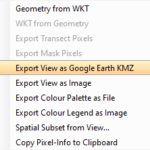 colored displacement map. Select Export View as Google Earth KMZ, and save the file.
2. Open Google Earth in your web browser. Wait for the web application to load.
3. Click the Bookmark Icon in the toolbar along the left side of the screen. Hovering over it will reveal the label My Places.
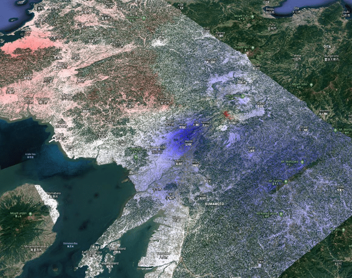
4. Click Import KML File > Open File and select your exported displacement map. Google Earth will overlay the map and zoom to the geographic area (Figure 14).

