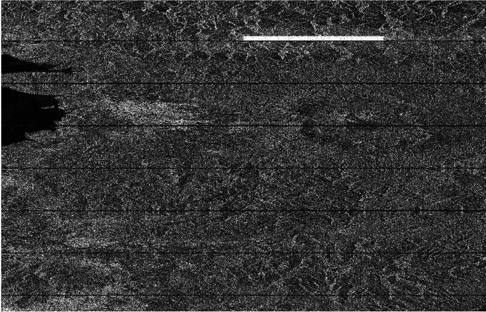
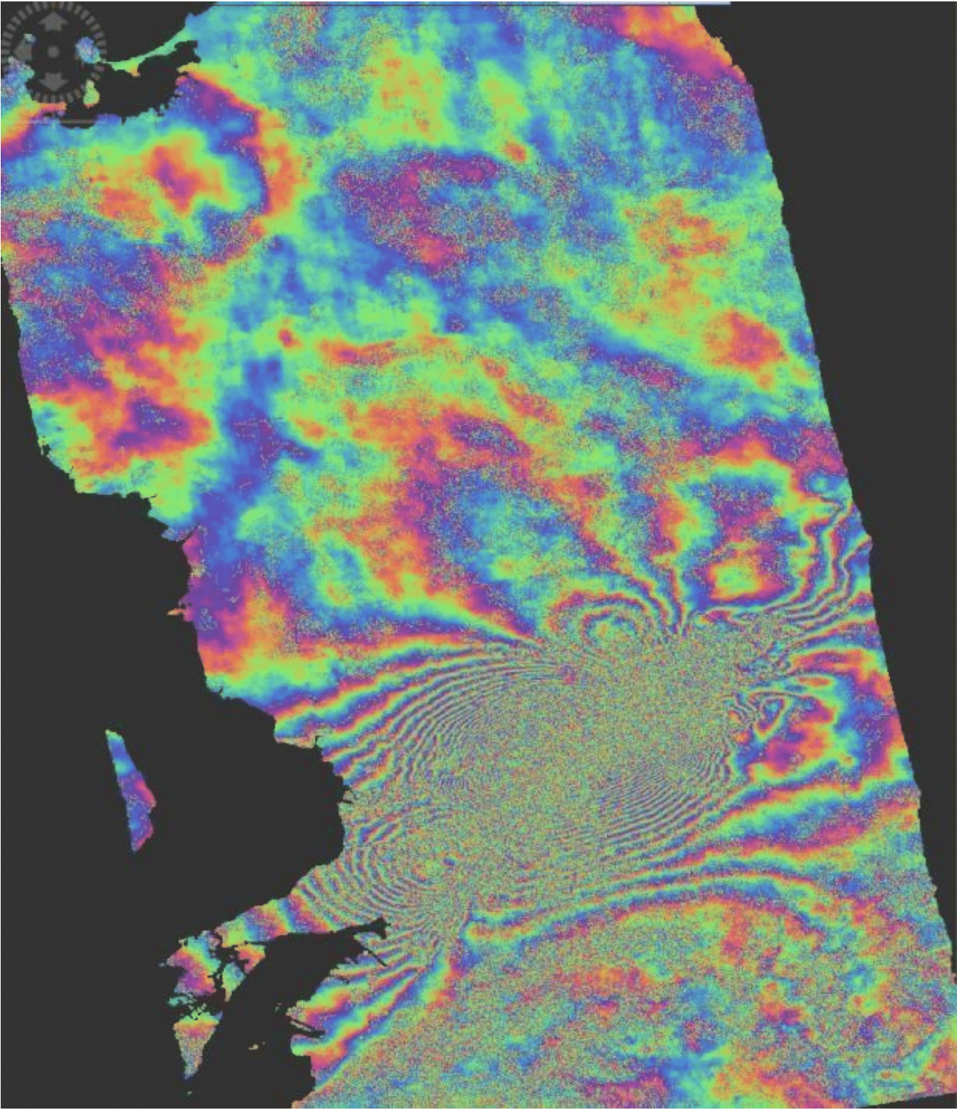
Deformation fringes related to the 2016 Kumamoto Earthquake show clearly after multi-looking and phase filtering were applied. Contains modified Copernicus Sentinel data 2016, processed by ESA.
Adapted from coursework developed by Franz J Meyer, Ph.D., Alaska Satellite Facility
■ Intermediate
Background
Introduction
Interferometric SAR processing exploits the difference between the phase signals of repeated SAR acquisitions to analyze the shape and deformation of the Earth surface. The principles and concepts of Interferometric SAR (InSAR) processing are not covered in this tutorial but may be found on the Data Recipes — Further Reading page.
The European Space Agency’s Sentinel-1A and Sentinel-1B C-band SAR sensors are delivering repeated SAR acquisitions with a predictable observation rate, providing an excellent basis for environmental analyses using InSAR techniques.
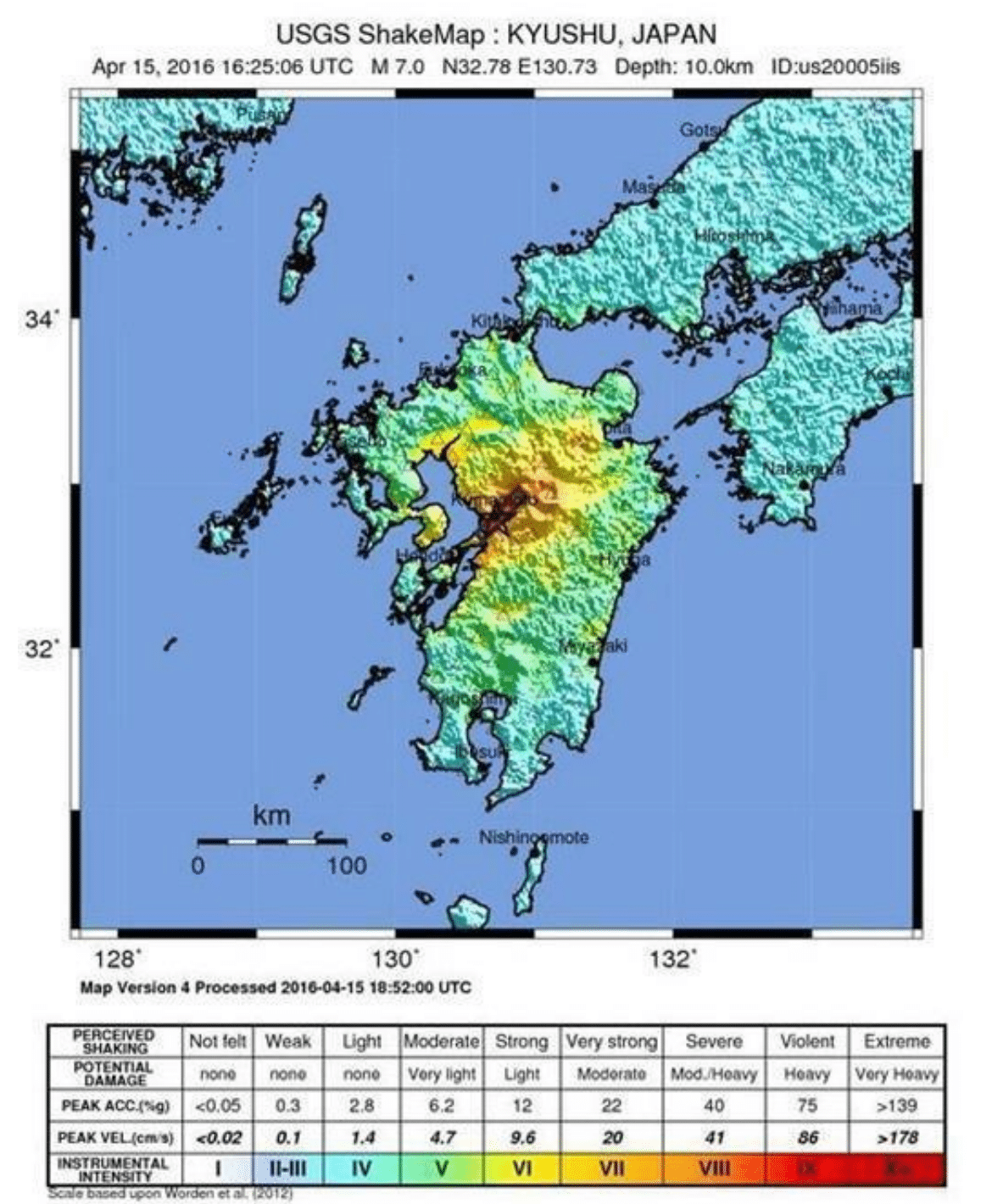
In this data recipe, for demonstration purposes, we will analyze a pair of Sentinel-1 images that bracket the devastating 2016 Kumamoto earthquake, whose 6.5 magnitude foreshock and 7.0 main shock devastated large areas around Kumamoto, Japan in April 2016. The image to the right shows the USGS ShakeMap associated with the 7.0 magnitude main shock, showing both the violence of the event and the location of the largest devastation.
A Word on Sentinel-1 Interferometric Wide Swath (IW) Data
The Interferometric Wide (IW) swath mode is the main acquisition mode over land for Sentinel-1. It acquires data with a 250km swath at 5m x 20m spatial resolution (single look). IW mode captures three sub-swaths using the Terrain Observation with Progressive Scans SAR (TOPSAR) acquisition principle.
With the TOPSAR technique, in addition to steering the beam in range as in ScanSAR, the beam is also electronically steered from backward to forward in the azimuth direction for each burst, avoiding scalloping and resulting in homogeneous image quality throughout the swath. A schematic of the TOPSAR acquisition principle is shown to the right.
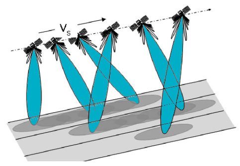
The TOPSAR mode replaces the conventional ScanSAR mode, achieving the same coverage and resolution as ScanSAR, but with nearly uniform image quality (in terms of Signal-to- Noise Ratio and Distributed Target Ambiguity Ratio).
IW Single Look Complex (SLC) products contain one image per sub-swath and one per polarization channel, for a total of three (single polarization) or six (dual polarization) images in an IW product.
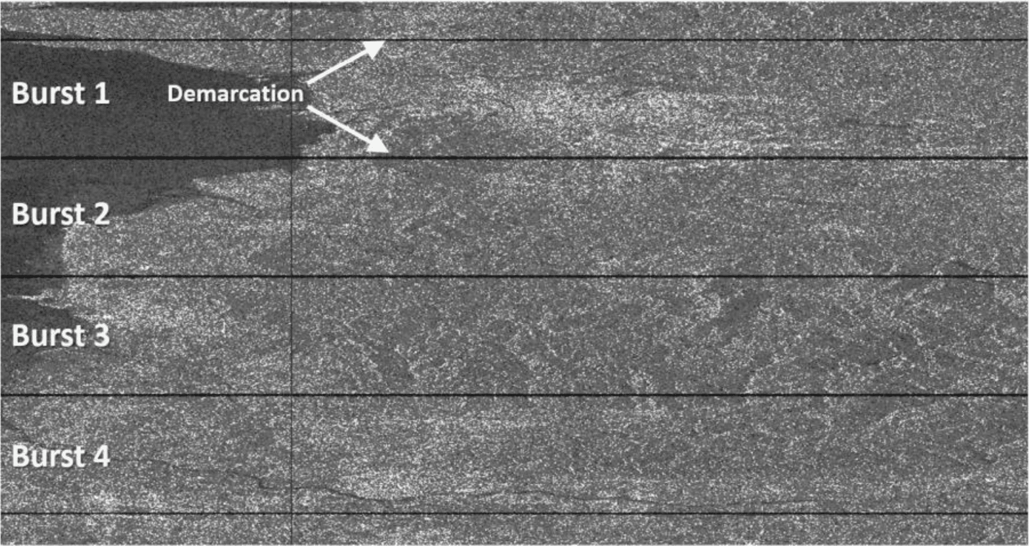
Each sub-swath image consists of a series of bursts, where each burst has been processed as a separate SLC image. The individually focused complex burst images are included, in azimuth-time order, into a single sub-swath image with black-fill demarcation in between, similar to ENVISAT ASAR Wide ScanSAR SLC products.
Sentinel-1 and the Kumamoto Earthquake
The sample images for this data recipe were acquired on April 8 and April 20, 2016, bracketing the fore and main show of the Kumamoto earthquake event. Hence, the phase difference between these image acquisitions captures the cumulative co-seismic deformation caused by both of these seismic events. The footprint of the Sentinel-1 images covers the areas most affected by the earthquake.

Prerequisites
Materials List
Note: You will be prompted for your Earthdata Login username and password, or must already be logged in to Earthdata before the download will begin.
Pre-event image sample:
Post-event image sample:
Move these files to a working directory for Sentinel-1 images in order to organize your processing workflow, but do not unzip the files.
System Requirements
Creating an interferogram using Sentinel-1 Toolbox is a very computer resource-intensive process and some steps can take a very long time to complete. Here are some hints to help speed things up and keep the program from freezing.
- Windows or Mac OS X
- Requires at least 16 GB memory RAM
- A Solid State Drive, as opposed to Hard Disk Drive, will speed up processing
- Close other applications
- Do not use the computer while a product is being processed
- Remove the previous product once a new product has been generated.
Steps for InSAR Processing
Opening Data in Sentinel-1 Toolbox
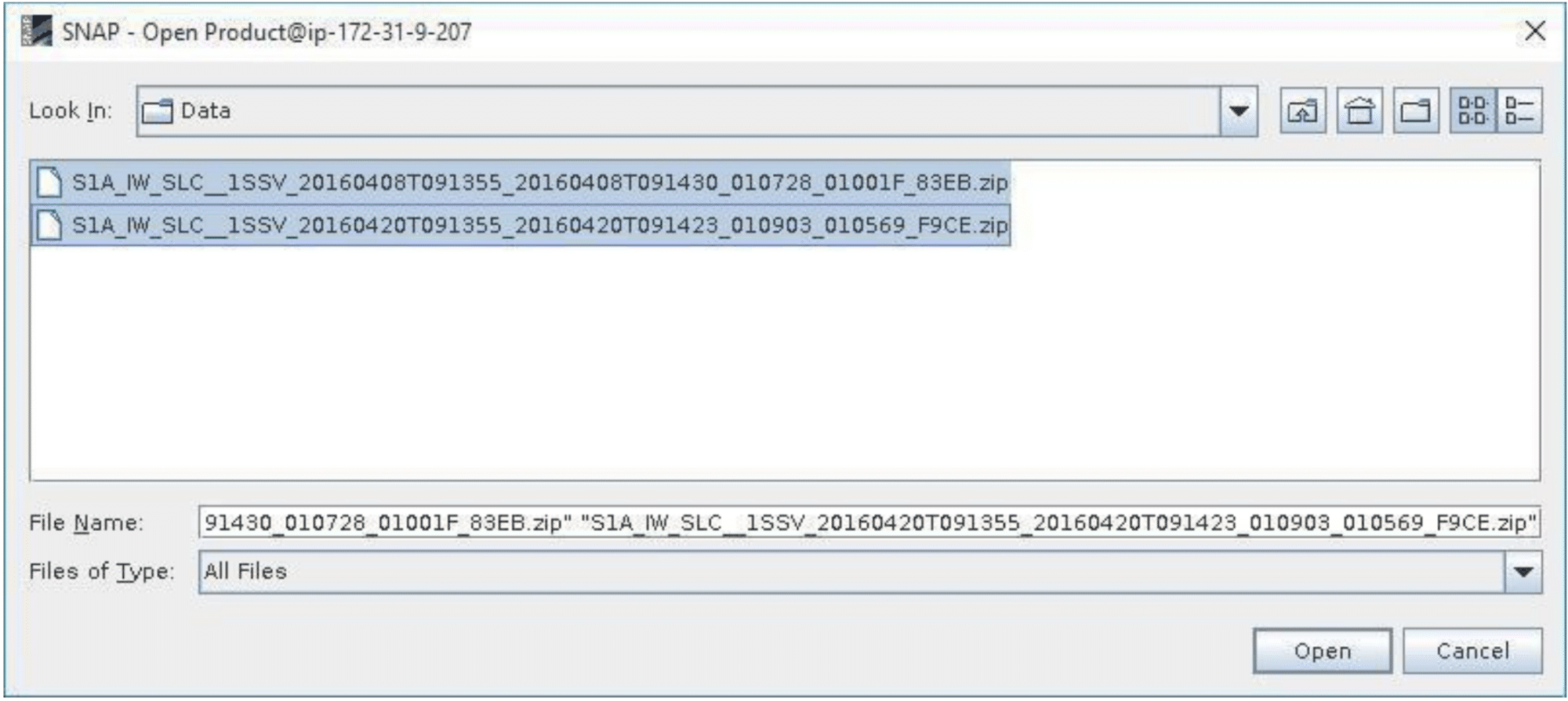
Start the Sentinel-1 Toolbox application (search for SNAP in your list of programs to find it). In order to perform interferometric processing, the input products should be two or more SLC products over the same area acquired at different times, such as the sample images provided in this tutorial.
Important: Sentinel-1 Toolbox works from the zip file format, so SLC files must remain zipped.
Open the Products
- Use the Open Product button in the top toolbar and browse to the location of the zipped Sentinel-1 Interferometric Wide (IW) SLC products.
- Select the two .zip SLC files. Click Open to load the files into Sentinel-1 Toolbox.
View the Products
In the Product Explorer window, you will see the products listed.
- Double-click on each product to expand the view.
- Double-click Bands to expand that folder for each product.
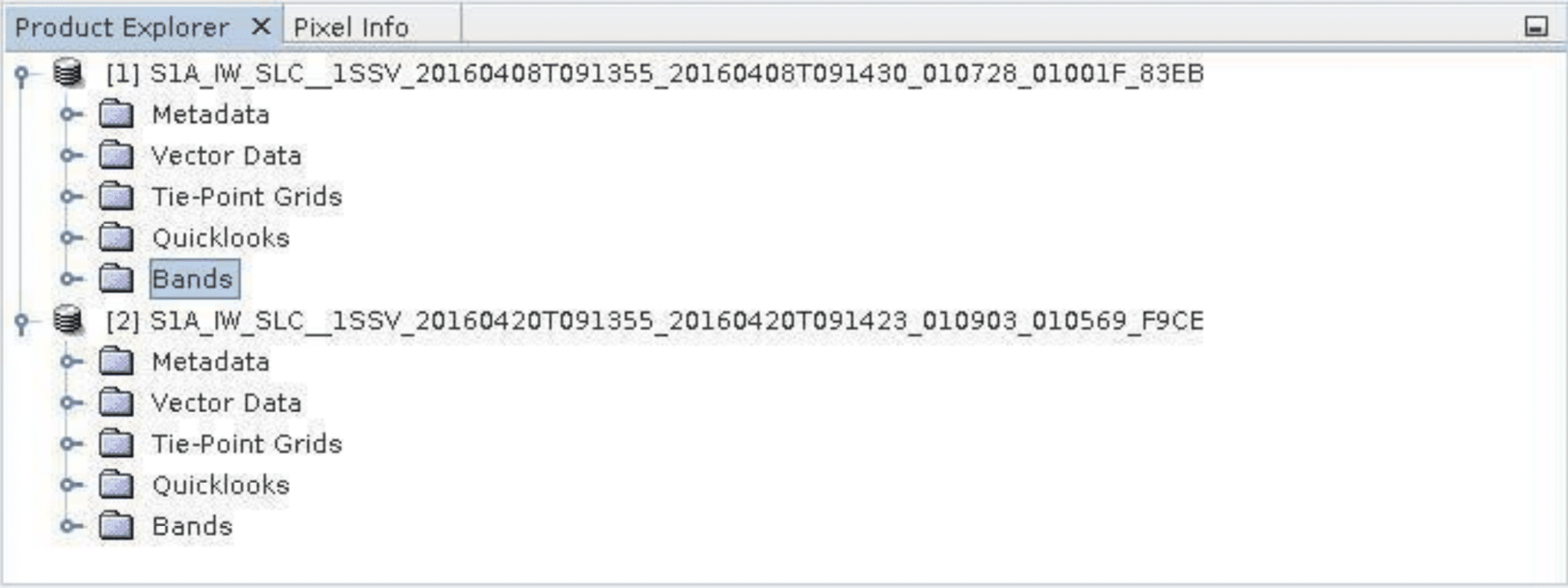
In the Bands folder, you will find bands containing the real (i) and imaginary (q) parts of the complex data. The i and q bands are the bands that are actually in the product, while the V(irtual) Intensity band is there to assist you in working with and visualizing the complex data.
Note that in Sentinel-1 IW SLC products, you will find three sub-swaths labeled IW1, IW2, and IW3. Each sub-swath is for an adjacent acquisition by the TOPS mode.
Note: To more easily follow the recipe, ensure that the _83EB SLC (earlier acquisition data) is listed as the first product and the _F9CE SLC (later acquisition data) is listed as the second product in the Product Explorer window.
Visualize a Band
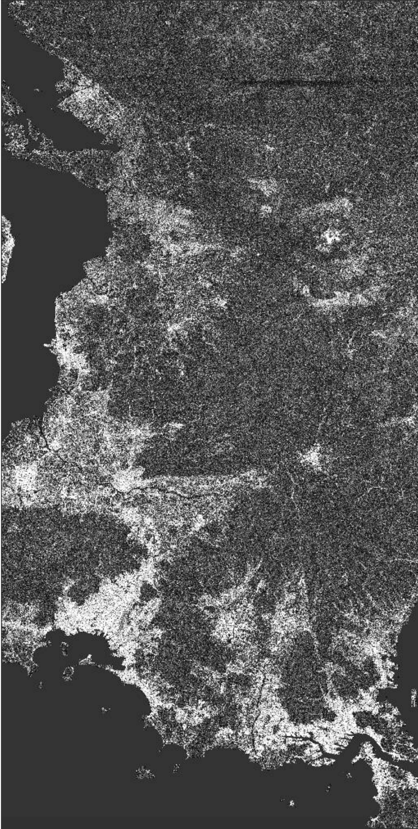
To view the data, double-click on the Intensity_IW1_VV band of one of the two images. Zoom in on the image and pan by using the tools in the Navigation window displayed below the Product Explorer window. Within a sub-swath, TOPS data are acquired in bursts. Each burst is separated by a demarcation zone. Any “data” within these demarcation zones can be considered invalid and should be zero-filled, but may also contain garbage values.
Coregister the Data
For interferometric processing, two or more images must be coregistered into a stack. One image is selected as the master and the other images are the “slaves.” The pixels in “slave” images will be moved to align with the master image to sub-pixel accuracy.
Coregistration ensures that each ground target contributes to the same (range, azimuth) pixel in both the master and the “slave” image. For TOPSAR InSAR, S-1 TOPS Coregistration is used.
TOPS Coregistration consists of a series of steps, which occur automatically once processing starts:
- Reading the two data products
- Selecting a sub-swath with TOPSAR-Split
- Applying precision orbit correction with Apply-Orbit-File
- Conducting a DEM-assisted Back-Geocoding Coregistration
Coregister the Images
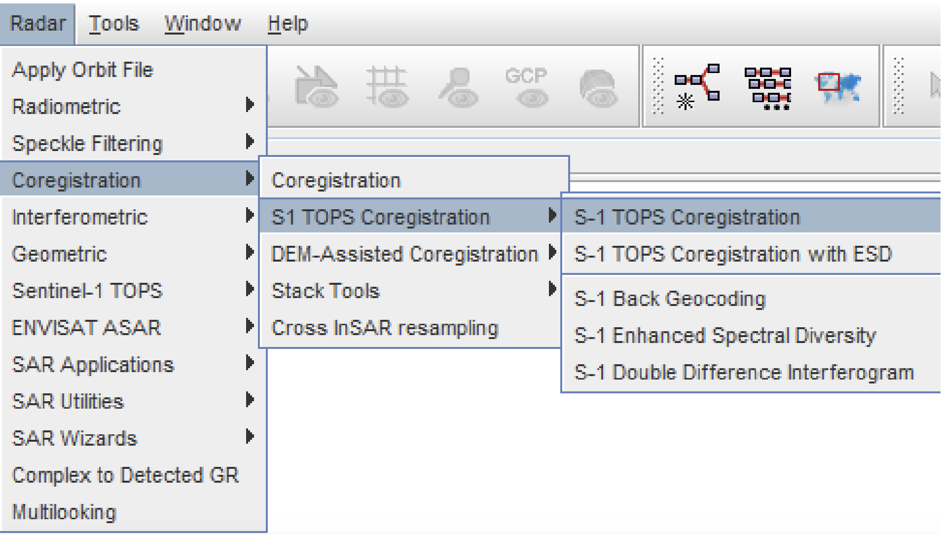
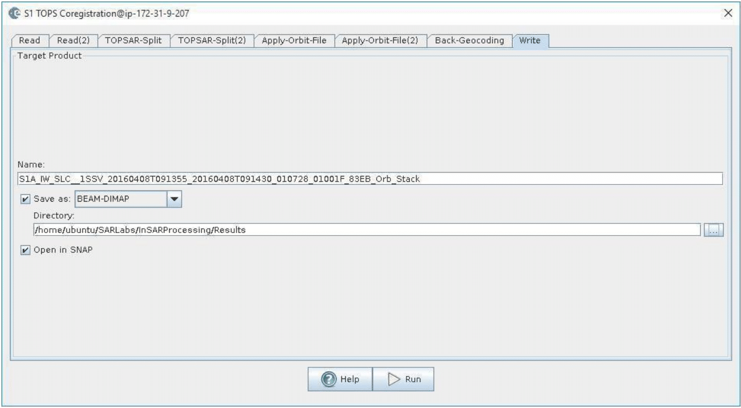
- From the Radar menu, select Coregistration > S1 TOPS Coregistration > S-1 TOPS Coregistration.
- A window will open, allowing you to set the parameters for the co-registration process.
- In the Read tab, select the first product. This should be the earlier of the two SLCs acquired on the 8th of April, 2016 (granule with suffix ID 83EB). This will be your “master” image.
- In the Read(2) tab, select the other product. This will be your “slave” image.
- In the TOPSAR-Split tabs, select the IW1 sub-swath for each of the products.
- In the Apply-Orbit-File tabs, select the Sentinel Precise Orbit State Vectors.
Orbit auxiliary data contain information about the position of the satellite during the acquisition of SAR data. Orbit data are automatically downloaded by Sentinel-1 Toolbox and no manual search is required by the user.
The Precise Orbit Determination (POD) service for Sentinel-1 provides Restituted orbit files and Precise Orbit Ephemerides (POE) orbit files. POE files cover approximately 28 hours and contain orbit state vectors at fixed time steps of 10-second intervals. Files are generated one file per day and are delivered within 20 days after data acquisition.
If Precise Orbits are not yet available for your product, you may select the Restituted orbits, which may not be as accurate as the Precise Orbits but will be better than the predicted orbits available within the product.
- In the Back-Geocoding tab, select the Digital Elevation Model (DEM) to use and the interpolation methods. The default is the SRTM 3 Sec DEM and this can be used for this tutorial. Areas that are not covered by the DEM or are located in the ocean may optionally be masked out.
- Select the option to Output Deramp and Demod Phase if you require Enhanced Spectral Diversity to improve the coregistration.
- In the Write tab, set the Directory path to your working directory.
- Click Run to begin coregistering the data. The resulting coregistered stack product will appear in the Product Explorer window with the suffix Orb_Stack.
Interferogram Formation and Coherence Estimation
The interferogram is formed by cross-multiplying the master image with the complex conjugate of the “slave.” The amplitude of both images is multiplied while their respective phases are differenced to form the interferogram.
The phase difference map, i.e., interferometric phase at each SAR image pixel, depends only on the difference in the travel paths from the SAR sensor to the considered resolution cell during the acquisition of each image.
Form the Interferogram
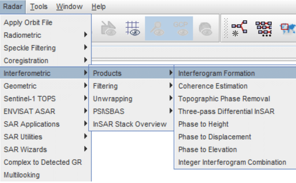
- Select stack [3] in Product Explorer and select Interferogram Formation from the Radar > Interferometric > Products menu.
Through the interferometric processing flow, we will try to eliminate other sources of error and be left with only the contributor of interest, which is typically the surface deformation related to an event.
The flat-earth phase removal is done automatically during the Interferogram Formation step. The flat-earth phase is the phase present in the interferometric signal due to the curvature of the reference surface. The flat-earth phase is estimated using the orbital and metadata information and subtracted from the complex interferogram.
- Keep the default values for Interferogram Formation, but confirm that the output Directory path is correct.
- Click Run.

Visualize Interferometric Phase
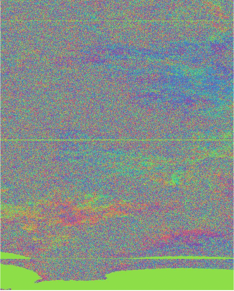
Once the interferogram product is created (product [4] in the Product Explorer, appended with Orb_Stack_ifg), expand the product and double-click the Phase_… band to visualize the interferometric phase (as in the Visualize a Band section). When zoomed in, you may still see the demarcation zones between bursts in this initial interferogram. This will be removed once TOPS Deburst is applied.
What it Means:
Interferometric fringes represent a full 2π cycle of phase change. Fringes appear on an interferogram as cycles of colors, with each cycle representing relative range difference of half a sensor’s wavelength. Relative ground movement between two points can be calculated by counting the fringes and multiplying by half of the wavelength. The closer the fringes are together, the greater the deformation on the ground.
Flat terrain should produce constant or only slowly varying fringes. Any deviation from a parallel fringe pattern can be interpreted as topographical variation.
TOPS Deburst
To seamlessly join all bursts in a swath into a single image, we apply the TOPS Deburst operator from the Sentinel-1 TOPS menu.
- Navigate to the Radar > Sentinel-1 TOPS menu.
- Select the S-1 TOPS Deburst option.
- Keep the default values, ensuring that product [4] (tagged _Orb_Stack_ifg) is selected as the Source and the output Directory path is correct.
- Click Run.
The resulting product will be appended with Orb_Stack_ifg_deb.

Topographic Phase Removal
To emphasize phase signatures related to deformation, topographic phase contributions are typically removed using a known DEM. In Sentinel-1 Toolbox, the Topographic Phase Removal operator will simulate an interferogram based on a reference DEM and subtract it from the processed interferogram.
- Navigate to the Radar > Interferometric > Products menu.
- Select the Topographic Phase Removal option.
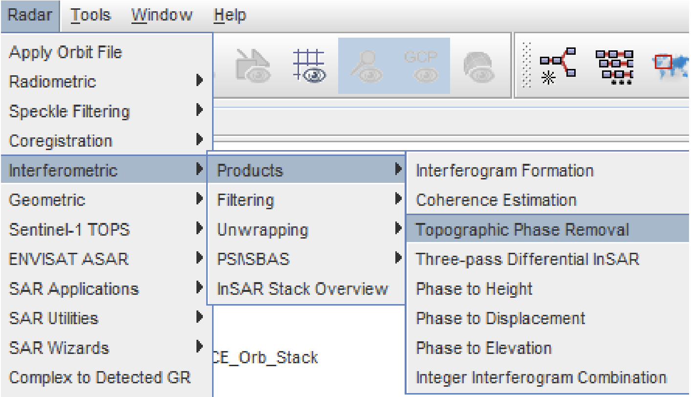
The Sentinel-1 Toolbox will automatically find and download the DEM segment required for correcting your interferogram of interest.
- Keep the default values (check that the source is product [5]) and click Run.
After topographic phase removal, the resulting product (appended with Orb_Stack_ifg_deb_dinsar) will appear largely devoid of topographic influence.
Multi-looking and Phase Filtering
Interferometric phase can be corrupted by noise from:
- Temporal decorrelation
- Geometric decorrelation
- Volume scattering
- Processing error
To be able to properly analyze the phase signatures in the interferogram, the signal-to-noise ratio will be increased by applying multi-looking and phase filtering techniques:
Multi-looking
The first step to improve phase fidelity is called multi-looking. Navigate to the Radar dropdown menu.
- Select the Multilooking option (bottom of the menu). A new window opens.
- Ensure that the source is set to product [6] (_dinsar) and the output Directory is correct.
- Click on the Processing Parameters tab.

Note: The coherence band (starting with coh_) will be essential if your intention is to unwrap the interferogram or create a deformation map. Coherence is used to verify the legitimacy of the derived phase data; typically data with coherence values less than 0.3 are thrown out. In this interferogram, coherence is highest in urban areas and lowest in vegetated areas.
- Use the Ctrl button to select the i, q, and coh bands from the list as the Source Bands to be multi-looked.
Because the phase band is virtual, it is only a temporary visualization of the interferogram. After multi-looking is performed, this band will disappear, but it will be restored in the following Goldstein Phase Filtering step.
- In the Number of Range Looks field, enter 6, which will result in a pixel size of about 26.5 meters.
In essence, multi-looking performs a spatial average of a number of neighboring pixels (in our case, 6×2 pixels) to suppress noise and proportion the image correctly. This process comes at the expense of spatial resolution.
- Click Run. The resulting product name is appended with Orb_Stack_ifg_deb_dinsar_ML.
Phase Filtering
In addition to multi-looking, we perform a phase filtering step using a state-of-the-art filtering approach.
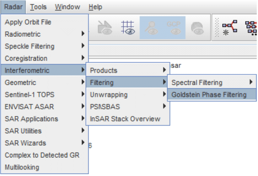
- Navigate to Radar > Interferometric > Filtering.
- Select Goldstein Phase Filtering.
- Ensure the source is set to product [7] (_ML) and that the output Directory path is correct.
- Keep the default values and click Run.
The resulting product name is appended with Orb_Stack_ifg_deb_dinsar_ML_flt.
After phase filtering, the interferometric phase is significantly improved, and the dense earthquake deformation-related ring pattern is now clearly visible.
This interferogram is now ready to be unwrapped. Instructions are available via ASF’s How to Phase Unwrap an Interferogram data recipe. If you came to this recipe via the Deformation Map Recipe, proceed with the steps iterated there. You can also continue with the geocoding and export steps if you just want a wrapped phase image.

Geocoding and Exporting in a User-defined Format
To make the data useful to geoscientists, the interferometric phase image needs to be projected into a geographic coordinate system using a DEM-assisted geocoding step. If your intention is to unwrap and further process the interferogram, this step should be skipped and performed at a later point.
Geocoding
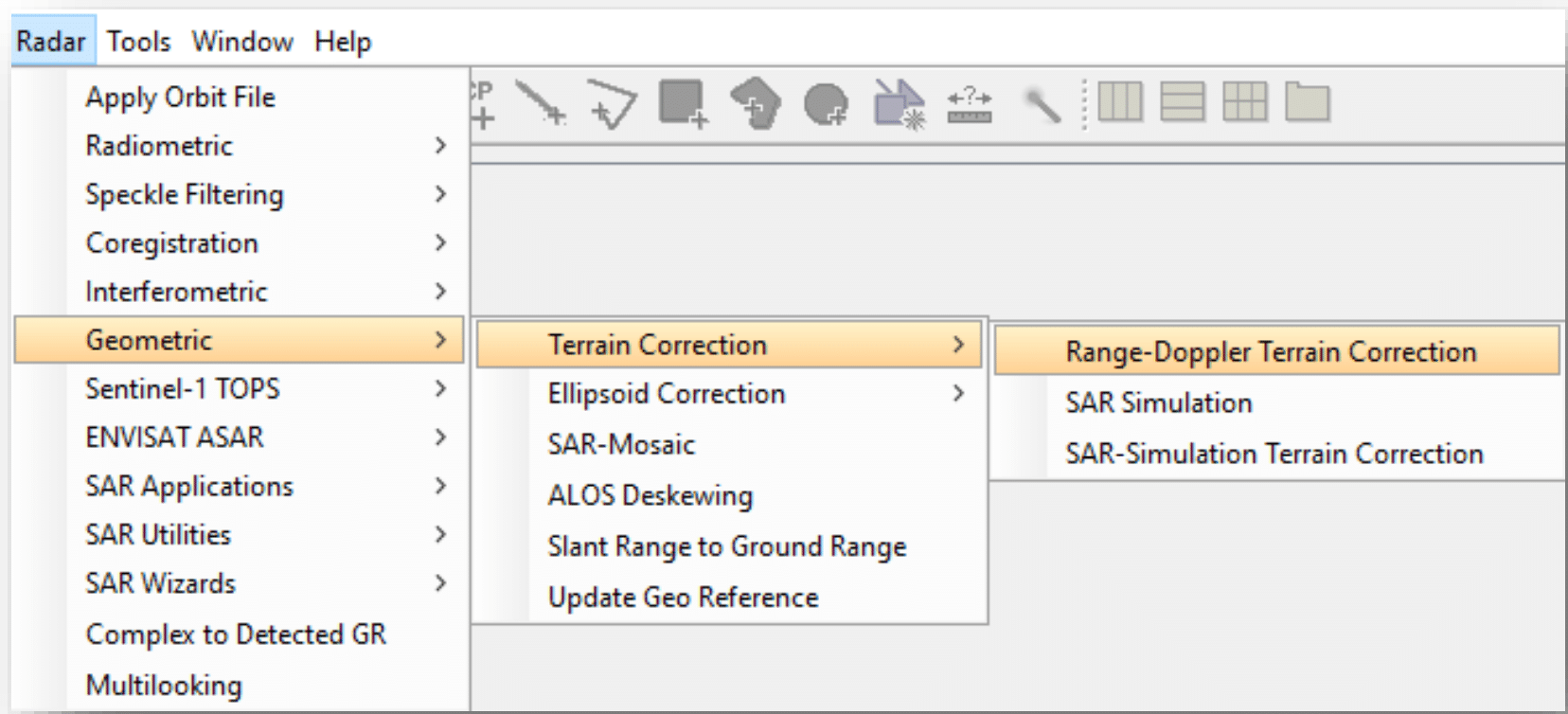
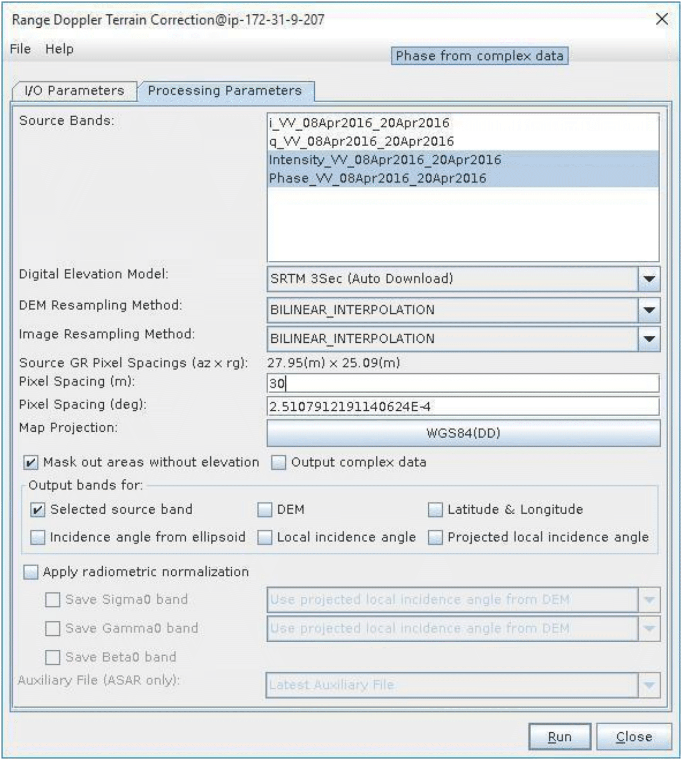
- Navigate to Radar > Geometric > Terrain Correction.
- Select the Range-Doppler Terrain Correction option.
- In the I/O Parameters tab of the Range-Doppler Terrain Correction window, select product [8] (or the product generated in the previous step) as the Source.
- In the Processing Parameters tab:
- Select the Phase band from the Source Bands list as the Source Band to be geocoded.
- Adjust the pixel spacing if desired.
- Click Run.
- If desired, re-run the process for the Intensity band.
The resulting product name is appended with Orb_Stack_ifg_deb_dinsar_ML_flt_TC. The resulting geocoded interferogram of subswath IW1 is located below.
Export Data
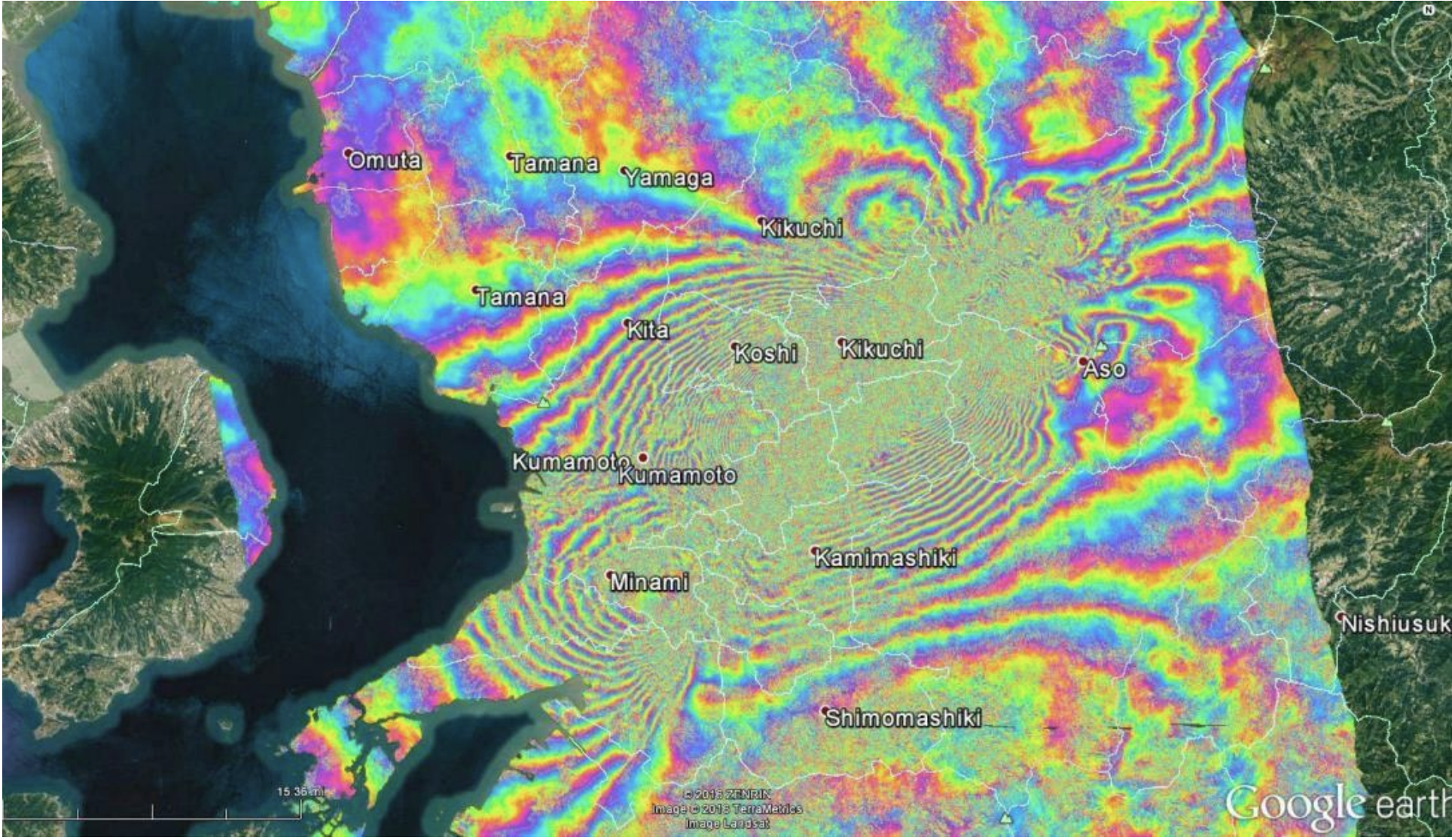
The final geocoded data can be exported from Sentinel-1 Toolbox in a variety of formats.
In addition to GeoTIFF and HDF5 formats, KMZ and various specialty formats are supported. The figure below shows a KMZ-formatted interferogram overlaid on Google Earth.
- Select the Geocoded product to export in the Product Explorer.
- To find the export options, select Export from the File menu.
- Note that if the Phase and Intensity bands were geocoded together, you will generate a 2-band GeoTIFF if you select that product.
- If you want to export a one-band product or generate a KMZ file, you will need to geocode the Phase band by itself and select that single-band product for export.
Optional — Combining Subswaths
Create a Geocoded Differential Interferogram of the Kumamoto Earthquake by Merging Subswaths IW1 and IW2:
To create the merged product, run the steps below, noting the new step.
- Run the Coregistration step: This time select IW2 in the TOPS Split and TOPS Split(2) operator tabs to coregister an InSAR pair for subswath IW2.
- The Subswath designation must match under the two TOPS Split tabs, or the process will not run.
- Make sure to create a new filename under the Write tab to avoid overwriting the IW1 stack result.
- Run the Interferogram Formation step: Using the new coregistered IW2 stack as input, create an IW2 subswath interferogram.
- Run the Debursting step: Deburst the IW2 interferogram.
- New Step — Merge Subswaths:
- To merge deburst SLC subswaths, go to the Radar > Sentinel-1 TOPS menu and select the S-1 TOPS Merge option.
- Select the deburst IW1 (Orb_Stack_ifg_deb) and deburst IW2 interferograms as inputs. Use the plus icon to browse from a directory, or the next button to add all the layers open in your project, then remove all but the two deburst products from the list.
- Run the remaining steps to create the final merged interferogram.
Interferogram Interpretation
The interferometric phase carries a wealth of information about surface deformation (strength and direction of motion) and the location of the surface rupture. The phase map is also a proxy for other earthquake-related parameters such as the energy released during an event and the amount of shaking experienced across the affected area.
Image Anomalies
SAR images sometimes suffer unavoidable radio frequency interference (RFI) from microwave sources on the ground transmitting in the same frequency. This is more common in maritime settings but it is also visible in the later image in this SLC pair. Consequently, this region on the image will generate inaccurate phase information. The coherence band will indicate this and provide a method for masking the anomaly out of interferogram or later products using band maths. Alternatively, selecting another SLC at a later point in time may decrease the coherence and quality of the entire interferogram.