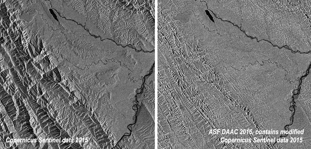
Before and after RTC: In this detail from the test granule below, mountains in Bolivia (left) appear stretched on one side and compressed on the other. RTC (right) moves pixels to unstretch the mountains and adjusts pixel values to subtract the effect of slopes on brightness. Credit left: Copernicus Sentinel data 2015. Credit right: ASF DAAC 2016, contains modified Copernicus Sentinel data 2015, processed by ESA.
Source: ASF Staff
■ Intermediate (Windows, OS X Unix): Use a script and the Sentinel Toolbox to correct distortions in multiple synthetic aperture radar (SAR) images
Background
Radiometric correction involves removing the misleading influence of topography on backscatter values. Terrain correction corrects geometric distortions that lead to geolocation errors. The distortions are induced by side- looking (rather than straight-down looking or nadir) imaging and are compounded by rugged terrain. Terrain correction moves image pixels into the proper spatial relationship with each other. Radiometric terrain correction combines both corrections to produce a superior product for science applications. This recipe is to support users who are comfortable working in the command line environment for post-processing SAR data. Note: Windows users with insufficient memory may see error messages.
ASF provides the python script procSentinelRTC_recipe.py to radiometrically terrain correct Sentinel-1A GRD data using the Sentinel-1 Toolbox software (S1TBX). This script uses a DEM file and a Sentinel-1A granule as inputs and creates terrain corrected GeoTIFFs of each polarization found in the granule, an incidence angle map, and a DEM file.
Prerequisites
Materials List
- Sentinel-1A GRD product (download from Vertex)
- Sample Granule (The images on the right use a detail from the full granule)
- (Optional) Digital Elevation Model (DEM) (available from sources including USGS Earth Explorer and Open Topography; choose projection in meters)
- Sentinel-1 Toolbox
- Python™ software package
- OSGeo4W shell (part of any recent version of QGIS)
- The procSentinelRTC_recipe.py script. Click the button below to download a zip file that contains the script and open-source software license.
Steps
- Create a directory (e.g., S1TBX_processing_directory) to house the Sentinel-1A GRD products (the .zip file) and the procSentinelRTC_recipe.py. The S1A zip file must be in the directory where python script is run, or Sentinel-1 Toolbox will fail to process the granule further.
- Download Sentinel-1A GRD data from ASF Vertex and move it to your Sentinel-1 Toolbox processing directory.
- Start with our sample granule.
- Download and install in your local environment the Sentinel-1 Toolbox package from ESA. On Windows paths with spaces cause difficulties, so the suggested location for the installation is c:\s1tbx.
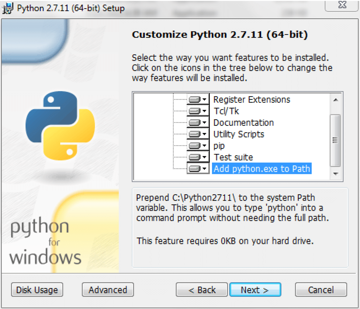
- Download and install in your local environment the Python™ 2.7 software package.
For Windows users, it is essential to Add python.exe to Path. A system administrator can help verify that the path is properly set in the environment variables for existing versions of Python.
- Download procSentinelRTC_recipe.py (part of this package found in the Data Recipe zip button) into your Sentinel-1 Toolbox processing directory.
- (Optional) Download external DEM as GeoTIFF if desired (DEMs are available from USGS Earth Explorer and OpenTopography; choose projection in meters), and place in Sentinel-1 Toolbox processing directory. Sentinel-1 Toolbox will download and apply a DEM from the SRTM mission if no additional DEM is provided by you.
- Download and install a recent version of QGIS, e.g., version 2.14 for the OSGeo4W shell.
- Modify the directory path name to reflect your Sentinel-1 Toolbox processing directory in the script, procSentinelRTC_recipe.py. If you are a Mac user, set the value of baseSNAP to be the location of the Sentinel-1 Toolbox GPT executable, i.e., baseSNAP = “/Applications/snap/bin/gpt”. If you are a Windows user, set the value of baseSNAP to the location of the Sentinel-1 Toolbox GPT executable, i.e., baseSNAP = “c:/snap/bin/gpt.exe”.
- For Windows users only: Start the OSGeo4W shell and change into the directory where the data recipe is stored.
- (Optional) The following options are available when running the script:
- -h, – -help show this help message and exit
- -r PS Pixel resolution — default = 10 meters
- -d DEM, – -dem=DEM External DEM filename
- -c, – -clean Clean intermediate files
- Run script
python procSentinelRTC_recipe.py [options] <S1A Zip File> <output directory>
Output
After the run is finished, there is a subdirectory named after the input data file as well as a “SAFE” directory containing the original data. Your data products are in the newly created file that matches your input file name. Your data products should be a GeoTIFF for each polarization of the SAR data (VV product or VV and VH products), a GeoTIFF of the DEM (DEM.tif) used for processing, and a GeoTIFF of the incidence angle map (INC.tif). All files are in the UTM projection.
cd TEMP
ls -1
S1A_IW_GRDH_1SDV_20150513T100637_20150513T100702_005901_0079A 1_E274
S1A_IW_GRDH_1SDV_20150513T100637_20150513T100702_005901_0079A 1_E274.SAFE
A listing of the sub-directory shows:
ls -1
S1A_IW_GRDH_1SDV_20150513T100637_20150513T100702_005901_0079A1_E274 S1A_IW_GRDH_1SDV_20150513T100637_20150513T100702_005901_0079A1_E274_OB_CAL.data S1A_IW_GRDH_1SDV_20150513T100637_20150513T100702_005901_0079A1_E274_OB_CAL.dim S1A_IW_GRDH_1SDV_20150513T100637_20150513T100702_005901_0079A1_E274_OB_CAL_TF.data S1A_IW_GRDH_1SDV_20150513T100637_20150513T100702_005901_0079A1_E274_OB_CAL_TF.dim S1A_IW_GRDH_1SDV_20150513T100637_20150513T100702_005901_0079A1_E274_OB_CAL_TF_TC.data S1A_IW_GRDH_1SDV_20150513T100637_20150513T100702_005901_0079A1_E274_OB_CAL_TF_TC_DEM.tif S1A_IW_GRDH_1SDV_20150513T100637_20150513T100702_005901_0079A1_E274_OB_CAL_TF_TC.dim S1A_IW_GRDH_1SDV_20150513T100637_20150513T100702_005901_0079A1_E274_OB_CAL_TF_TC_GVH.tif S1A_IW_GRDH_1SDV_20150513T100637_20150513T100702_005901_0079A1_E274_OB_CAL_TF_TC_GVV.tif S1A_IW_GRDH_1SDV_20150513T100637_20150513T100702_005901_0079A1_E274_OB_CAL_TF_TC_INC.tif S1A_IW_GRDH_1SDV_20150513T100637_20150513T100702_005901_0079A1_E274_OB.data S1A_IW_GRDH_1SDV_20150513T100637_20150513T100702_005901_0079A1_E274_OB.dim
The .data and .dim files are in native Sentinel-1 Toolbox format. The file extensions show the processing that was performed:
| OB | Precise orbit applied |
| CAL | Calibrated |
| TF | Terrain Flattening |
| TC | Terrain Correction |
How it Works
The procSentinelRTC_recipe.py script makes 4 calls to the Sentinel-1 Toolbox software gpt executable, followed by a conversion of the files from the ENVI format into GeoTIFFs. The steps are as follows:
- Apply precise orbit information to the input file via automatic download.
- Radiometrically calibrate the image to Beta0 (the terrain flattening algorithm requires Beta0 input).
- Radiometrically “flatten” the image, reducing terrain-induced radiometric variations.
- Geometrically correct the image, reducing terrain-induced distortions.
gpt Terrain-Correction -PsaveDEM=true – PsaveProjectedLocalIncidenceAngle=true \
-PmapProjection=EPSG:<UTMCODE> – PpixelSpacingInMeter=<pixsiz>
(Optional) View the RTC Image in a GIS Program
Note the Gamma0 file type that the Sentinel-1 Toolbox RTC process produces is excellent for statistical comparisons, but can appear very dark. To view a lighter version of the image in a GIS environment, see the ASF data recipes How to View Radiometrically Terrain-Corrected (RTC) Images in QGIS or How to View Radiometrically Terrain-Corrected (RTC) Images in ArcGIS.
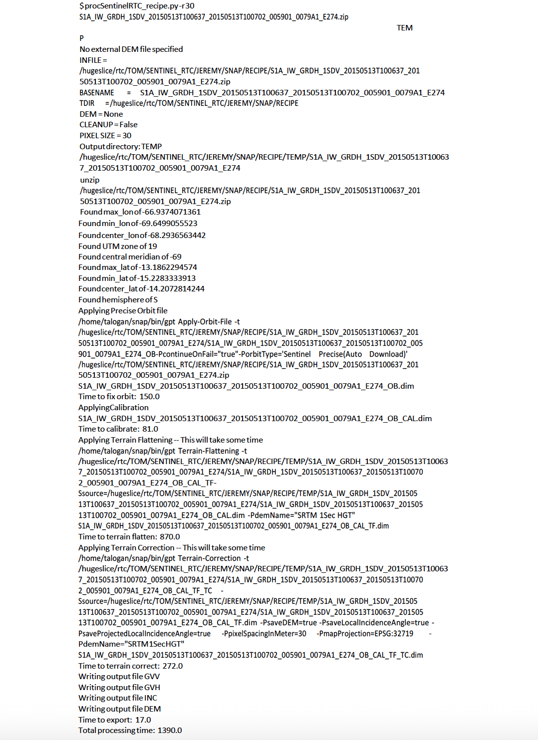
Example Run