
Summary
During its brief 106-days of lifetime, the Seasat-1 spacecraft, launched on June 28, 1978, by NASA’s Jet Propulsion Laboratory (JPL), collected information on sea-surface winds, sea-surface temperatures, wave heights, internal waves, atmospheric water, sea ice features, ice sheet topography, and ocean topography. This was the first JPL mission to study Earth with the use of imaging radar.
While much of the data collected in the USA was processed optically, only 150 scenes had been digitally processed by March 1980. In fact, only an estimated 3 to 15 percent of Seasat data was ever digitally processed.
ASF’s Seasat holdings have been captured to disk and the raw telemetry data have been decoded and filtered into readily processable signal files. In addition, engineers at ASF have developed the ASF Seasat Processing System (ASPS), a robust package that generates detected georeferenced products in both HDF5 and GeoTIFF formats with ISO 19115 compliant metadata stored as XML. The beta version products are being processed and released over the summer of 2013.
1. Source/Platform or Data Collection Environment Overview
Source/Platform Name, Source/Platform Acronym
Ocean Dynamics Satellite/Seasat
Source/Platform Introduction
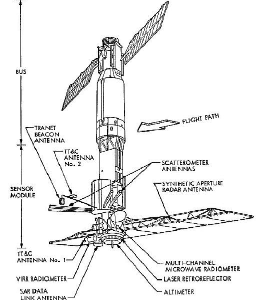
Seasat supported five sensors: ALT (radar altimeter), SMMR (Scanning Multichannel Microwave Radiometer), SAR (Synthetic Aperture Radar), SASS (Seasat-A Scatterometer System), and VIRR (Visible and Infrared Radiometer). Seasat was in a near-circular, polar orbit at an altitude of 805 kilometers and at an inclination of 108 degrees. The satellite orbited the Earth 14 times daily and covered 95 percent of the world’s oceans every 36 hours. On October 10, 1978, the satellite suffered a massive short circuit in its electrical system and stopped functioning.
During operation, Seasat utilized two basic orbital configurations. The initial observational phase was a 17-day repeat cycle. On September 8, the satellite was maneuvered into an exact 3-day repeat.
Source/Platform Program Management
Seasat was a NASA/Jet Propulsion Laboratory Earth observation mission. Although Seasat operated five onboard sensors, only the Synthetic Aperture Radar (SAR) data are covered herein. Jet Propulsion Laboratory managed this sensor.
Source/Platform Mission Objectives
Seasat was specifically designed to study oceanographic phenomena. The mission’s purpose was to help determine the requirements for an operational ocean remote-sensing satellite system.
Source/Platform Parameters
Seasat was launched on June 26, 1978, from the Vandenberg Air Force Base, California. The Seasat launch vehicle, Atlas-Agena, provided attitude control, power, guidance, telemetry, and command functions. A sensor module was attached to the Agena and carried the payload of five microwave instruments and their antennas. Together, the two modules measured 21 meters long and 1.5 meters in diameter. Once in orbit and after burnout of the Agena stage, the Seasat spacecraft weighed 2300 kilograms.
Attitude Characteristics
Atlas-Agena, the Seasat launch vehicle, provided attitude control for the satellite. In orbit, Seasat appeared to stand on end, with the sensor and communications antennas pointing toward Earth and the Agena rocket nozzle and solar panels pointing toward space. Seasat was stabilized by a momentum wheel/horizon sensing system.
SAR (Synthetic Aperture Radar) Sensor
The SAR onboard Seasat monitored the global surface wave field and polar sea ice conditions, providing information on ice caps, snow coverage, and coastal regions. The experiment operated at L-band (1.275 GHz) with a 100-km swath and provided 25-m vertical resolution. About 42 hours of data were recorded.
| Seasat SAR Sensor Parameters | |
|---|---|
| Polarization | HH |
| Look direction | Right |
| Footprint | 100 km X 15 km |
| Image frame size | 100 km X 100 km |
| Image Resolution | 25 m |
| Number of looks | 4 |
| Bandwidth | 19 MHz |
| Slant range resolution | 6.6 m |
| Ground range resolution | 17-23 m (based on incidence angle) |
| Frequency | 1275 MHz - L-Band |
| Radar Wavelength | 23.5 cm |
| Pulse duration | 33.8 microseconds |
| Sampling Rate | 45.53 MHz |
| Sampling Time | 21.97 nS |
| Sampling Window Duration | 288 microseconds |
| Incidence Angle | 23 +/- 3 degrees |
| Pulse Repetition Frequency | 1647 Hz |
| Data sample size | 5-bits |
2. Data Acquisition and Historical Processing
Data were transmitted from the satellite in three separate streams: 25-kbps real-time stream containing instrument data from ALT, SASS, SMMR, and VIRR and all engineering subsystem data, an 800-kbps playback stream of recorded real-time data, and a 20-MHz analog SAR instrument data stream.
Seasat was not equipped with an onboard recorder, so in order to collect data during the mission, three U.S. and two international ground stations downlinked data from the satellite in real time: Fairbanks, Alaska; Goldstone, California; Merritt Island, Florida; Shoe Cove, Newfoundland, and Oakhanger, United Kingdom.
SAR data from Seasat were acquired digitally, and most of the data were optically processed into survey data products, available on 70-mm film. The Seasat 100-km swath data were processed into four 25-km wide products at JPL. A small percentage of the data were digitally processed. These products contain the complete 100-km wide swath of data. (JPL’s Seasat digital processor operated from 1978 to 1982, converting approximately 10 percent of the total Seasat data set to precision data. JPL currently has no capability to process additional SAR data from Seasat.)
After acquisition, the data were originally archived on 39-track raw data tapes. Years later, to ensure the preservation of the data, those tapes were duplicated in 1988 and again in 1999. During the second transcription, the raw telemetry data were transferred onto twenty-nine more modern SONY SD1-1300L 19 mm tapes. It is from these 13-year-old tapes that ASF’s Seasat products were processed.
3. Data Description
Spatial Characteristics
Seasat products are detected amplitude images stored as 4-byte floating point numbers. The detected products are 8,000 lines by 8,000 samples with 12.5 meter ground range spacing, giving a total product size of 100 km2. The data is not calibrated.
Data Naming Convention
The ASF Seasat products are centered at ESA standard nodes. The naming convention for Seasat products is as follows:
SS_ooooo_STD_Fffff
Where ooooo is the five digit orbit number of Seasat platform at time of imaging and ffff is the four digit ESA node number signifying the center latitude of the product. For node 0-1800 the center latitude is (node * 0.05) degrees, while for nodes 1801-3600 the center latitude is 180.0 – (node * 0.05) degrees.
HDF5 Product
HDF5 uses two primary structures – groups and datasets – to organize data in a hierarchical structure. The data group contains the SAR data as backscatter values in the HH layer. In order to provide basic geolocation information, two additional layers, latitude and longitude, are added. They contain geographic coordinates for every pixel in the image. The time variable completes the compliance to the Climate and Forecast (CF) metadata conventions (CF Conventions Committee, 2013).
The structure within the metadata group was modeled after the TerraSAR-X metadata (Astrium, 2013). The generalHeader section defines very basic metadata such as mission and data source. The instrument section summarizes radar parameters and settings. The satellite flight path with its orbital parameters is described in the platform section. The processing section provides vital information about Doppler as well as about processing parameters and flags. All product components are included in the productComponents section. The general product information is given in the productInfo section, while the SAR specific is stored in the productSpecific section. Finally, the setup section provides details about data ordering and processing. Users are advised that the Seasat HDF5 products may have substantial geolocation errors. The ASF Seasat HDF5 products have the file extension .h5
GeoTIFF Product
GeoTIFF is a public domain metadata standard that allows georeferencing information to be embedded within a TIFF file. The GeoTIFF data products are geocoded to the Universal Transverse Mercator (UTM) map projection, using the zone that best represents the data’s geolocation. The original 12.5 m pixel size and the floating-point values of the ground range HDF5 products are kept in the GeoTIFF format. Because this product type does not require additional geographic information, it only contains a single layer of SAR data and is, therefore, considerably smaller than the HDF5 product. Users are advised that the Seasat GeoTIFF products may have substantial geolocation errors. The ASF Seasat GeoTIFF products have the file extension .tif.
Standard Product Inclusions
In addition to either an HDF5 or a GeoTIFF format image, each Seasat product package will contain the following files:
- SS_00351_STD_F1137.iso.xml – The development of XML metadata that is entirely compliant to ISO 19115 and other related standards (NOAA EDM, 2013) is work in progress.
- SS_00351_STD_F1137.jpg – Browse image of the product data. The file is down sampled to 1/8th of the original pixel spacing (100 meters) and saved in compressed JPEG format. The file is in swath orientation.
- SS_00351_STD_F1137.kml – Keyhole Markup Language (KML) is an XML-based markup language designed to annotate and overlay visualizations on various two-dimensional, Web-based online maps or three-dimensional Earth browsers (such as Google Earth). These KML files contain a bounding box representing the spatial coverage of the product. Please be aware that some Seasat images display substantial geolocation errors.
- SS_00351_STD_F1137.qc_report – During production, all of the Seasat imagery created by ASF went through a quality control procedure to screen for various image and processing anomalies. The qc_report file contains the results of that QC process, including any individual comments that were made about an image during examination.
- SS_00351_STD_F1137.xml – The same metadata structure as is stored in the HDF5 file is saved as an XML file for ease of access and parsing the information.
4. Data Manipulations
Raw Data Decode
During decoding of the raw Seasat SAR telemetry, several data manipulations were required in order to make the signal data usable in an automated fashion.
- Decoded range lines are formed from a variable number of minor frames. Every signal file decoded had errors in these minor frame numbers. In the worst file, 17% were incorrect in some manner. Thus, the ASF Seasat decoder had to use heuristics to try to properly find the start of each range line that was formed.
- Partial lines occurred in 87% of the data files decoded by ASF. Each of these partial lines was zero-filled to create full range lines. Only those decoded swath files that contained less than 4.5% partial lines were processed into products. Even then, only 32 of 1,346 cleaned signal files showed more than 1% partial lines, and, no visual anomalies resulting from partial lines were observed in the data.
Median Filtering Raw Data
Seven metadata parameters were median filtered to pull out the most commonly occurring value: station code, day of year, clock drift, delay to digitization, least significant digit of year, bits per sample, and PRF rate code. Prior to this, these metadata fields were unusable.
Time Filtering Raw Data
Decoded satellite time values were fraught with various errors – some systematic, some due to degradation or transcriptions. 728 datasets (50%) had time gaps. One file had as many as 1820 different gaps. 295 files (20%) showed a sticking time clock resulting in “stair step” timing errors. Thus, the time values had to be filtered in many successive stages to create linear time values that were accurate for the data collection period.
The final time of imaging was determined using these filtered times plus the median filtered times found in the satellite cock drift metadata field. In the end, missing lines were filled with random values in 494 out of 1346 swath files. Although the worst file that was saved had 136 gaps filled, only 34 files had 10 or more gaps while 288 files had only one or two gaps in them.
Geolocation - Slant Range Adjustment
ASF has attempted to make first order corrections to the geolocations of their Seasat products. Two state vector sources were examined. The Seasat precise orbits solutions from the NASA Goddard Space Flight Center were used to create products. Satellite imaging times were filtered as accurately as possible. Although ASF has not undertaken a thorough analysis of geolocation accuracies, it was noted that Seasat geolocations usually show an across-track error. To adjust for this, a -1000 meter slant range shift was introduced into the products when calculating georeferencing information. Users are advised that when attempting to recreate the geolocations stored in either the HDF5 or the GeoTIFF products, this -1000 meter slant range shift must be taken into account.
Spectral Filtering
Early in data exploration, the power spectra of Seasat signal data were analyzed. Rather than show the standard relatively flat peak, the Seasat spectra show tones that should not be present in raw data. To remove this frequency interference, the notch filter functionality of ROI was modified to remove up to twenty unwanted caltones. All values greater than 1.5 standard deviations from the mean spectral value were gathered and sorted. Closely neighboring caltones were culled, creating the final list of caltones that were removed.
5. Data Quality Issues
Far Range Samples
The decision was made to create 100 km wide swaths even though this may introduce a few pixels in the far range that do not contain the contributions from a full 1,539 raw samples. As a result, users may notice slight darkening in the last 824 range samples in some images. This is intentionally done in order to create square Seasat products.
Sensor Anomalies
No data
Many of the original swaths start with no data being collected, introduce real data after some number of lines, and end the datatake with another patch of no data collection. This means that swaths contain both invalid and valid data. Since the bit fields that may have given information on whether or not the satellite was actually imaging were unreliable, ASF chose to process all of the data in each swath. Products that contain more than 50% were kept and made available in the ASF datapool. Thus, some of the ASF Seasat products contain areas of no valid SAR data that is easily identified by blackness resulting from having no data to focus during processing.
Calibration Pulse
During the start of the Seasat mission, when engineers were still testing system parameters, a calibration pulse was introduced into the raw signal data. Unfortunately, since the mission was cut so short by a power failure, this means that much of the Seasat data has an embedded calibration pulse. This pulse, when focused, forms a bright white line in the azimuth direction, somewhere near the middle of the swath. Preliminary examination of the calibration pulse shows that it can be removed – it is ASF’s intention to do so in future releases of the Seasat products.
Dashes
Another signal was embedded into the Seasat raw data. This one creates a set of short lines across the range direction of an image when focused. It has been verified that this signal is a real occurrence in the raw data. It is not known what intent of this signal was. It is noted that whenever this signal is present in the data, the calibration pulse is not. Although often the calibration pulse precedes and follows a section of dashes in an image, it also appears in data that has no calibration pulse. It is unclear if this signal can be removed from the raw data in a future release of the ASF Seasat products, but it will be examined for feasibility.
Attenuation
Some of the ASF Seasat products have extreme across-track attenuation. The effect is that the near range of the image is very bright, while the far range is quite dark. It was initially thought this had to do with the gain control on the satellite (which was one of those unreliable bit fields). However, in discussions with JPL engineers, it is possible that this was caused by incorrect delay to digitization settings during the first part of the Seasat mission. In any case, this effect probably can never be removed from the imagery, only noted as a data quality issue.
Image Anomalies
Banding
Banding across SAR imagery is a fairly common occurrence and can be the result of atmospheric effects or poor data. Some banding was noticed in the ASF Seasat products.
Along-Track Streaks
Much, if not all, of the Seasat imagery, shows some amount of along-track streaking. Although ASF removed some of these streaks using the range spectra filtering, some remains.
Across-Track Streaks
In addition to the along-track streaks, across-track streaks also occur. Typically these are lines across the imagery, often bent in one direction or another. This bending results from the range migration portion of the SAR focusing algorithm.
Missing Lines
When the Seasat data was first decoded, over half of the datasets showed time gaps. In the end, missing lines were filled with random values in 494 out of 1346 swath files. Although the worst file that was saved had 136 gaps filled, only 34 files had 10 or more gaps while 288 files had only one or two gaps in them.
The ensure users are fully aware of data anomalies that may cause analysis issues, any missing lines that occur within the raw data used to focus a product are annotated in the XML metadata files provided with the products.
<productQuality>
<rawDataQuality>
<polLayer>HH</polLayer>
<beamID>SAR</beamID>
<numGaps>3</numGaps>
<gap num=”1″>
<start>7607</start>
<length>11</length>
<fill>RANDOM</fill>
</gap>
<gap num=”2″>
<start>7791</start>
<length>10</length>
<fill>RANDOM</fill>
</gap>
<gap num=”3″>
<start>7865</start>
<length>29</length>
<fill>RANDOM</fill>
</gap>
<gapSignificanceFlag>false</gapSignificanceFlag>
<missingLinesSignificanceFlag>false</missingLinesSignificanceFlag>
<bitErrorSignificanceFlag>false</bitErrorSignificanceFlag>
<timeReconstructionSignificanceFlag>false</timeReconstructionSignificanceFlag>
</rawDataQuality>
Data Gap Information in XML: Each time that a data gap occurs in the raw data used to create an ASF Seasat product, it is annotated inside the XML metadata file.
Geolocation Errors
The data quality group at ASF examined six different sites for geolocation accuracy. Each image’s geolocations were matched against the same feature in an ALOS PALSAR image.
The examined geolocation errors are within 1 kilometer in 4 out of 6 cases (see table). Users are advised that geolocation offsets of up to several kilometers have been observed in some products.
| Site Location | Observed Geolocation Offset |
|---|---|
| Albany, OR | 1300.7 |
| Big Delta, AK | 908.8 |
| Datchet, England | 812.5 |
| Dallas, TX | 1611.8 |
| Milton, LA | 351.9 |
| Apalachicola, Florida | 152.1 |
Geolocation Analysis: The ASF data quality group compared locations in Seasat images with locations in corresponding ALOS PALSAR imagery, examining six sites.
Although ASF has not undertaken a thorough analysis of geolocation accuracies, it was noted that Seasat geolocations usually show an across-track error. To adjust for this, a negative 1000 meter slant range shift was introduced into the products when calculating georeferencing information. Users are advised that when attempting to recreate the geolocations stored in either the HDF5 or the GeoTIFF products, this -1000 meter slant range shift must be taken into account.
6. Using HDF5 Products
The Seasat HDF5 products are currently supported to different degrees by a number of software packages that can be used to investigate and visualize the data.
GDAL
The Geospatial Data Abstraction Library (GDAL) helps to explore the general contents of the Seasat HDF5 data. The gdalinfo tool summarizes the data structure in the file.
$ gdalinfo -nomd SS_00788_STD_F3003.h5
Driver: HDF5/Hierarchical Data Format Release 5
Files: SS_00788_STD_F3003.h5
Size is 512, 512
Coordinate System is `’
Subdatasets:
SUBDATASET_1_NAME=HDF5:”SS_00788_STD_F3003.h5″://data/HH
SUBDATASET_1_DESC=[8000×8000] //data/HH (32-bit floating-point)
SUBDATASET_2_NAME=HDF5:”SS_00788_STD_F3003.h5″://data/latitude
SUBDATASET_2_DESC=[8000×8000] //data/latitude (32-bit floating-point)
SUBDATASET_3_NAME=HDF5:”SS_00788_STD_F3003.h5″://data/longitude
SUBDATASET_3_DESC=[8000×8000] //data/longitude (32-bit floating-point)
Corner Coordinates:
Upper Left ( 0.0, 0.0)
Lower Left ( 0.0, 512.0)
Upper Right ( 512.0, 0.0)
Lower Right ( 512.0, 512.0)
Center ( 256.0, 256.0)
The gdal_translate tool can extract the SAR data out of the structure and store it into more versatile GeoTIFF.
$ gdal_translate HDF5:”SS_00788_STD_F3003.h5″://data/HH SS_00788_STD_F3003_geo.tif
Input file size is 8000, 8000
0…10…20…30…40…50…60…70…80…90…100 – done.
The newly generated GeoTIFF contains control points extracted from the latitude and longitude layers of the original HDF data.
Driver: GTiff/GeoTIFF
Files: SS_00788_STD_F3003_geo.tif
Size is 8000, 8000
Coordinate System is `’
GCP Projection =
GEOGCS[“WGS 84”,
DATUM[“WGS_1984”,
SPHEROID[“WGS 84”,6378137,298.257223563,
AUTHORITY[“EPSG”,”7030″]],
AUTHORITY[“EPSG”,”6326″]],
PRIMEM[“Greenwich”,0],
UNIT[“degree”,0.0174532925199433],
AUTHORITY[“EPSG”,”4326″]]
GCP[ 0]: Id=1, Info=
(0.5,0.5) -> (90.1664428710938,29.2081909179688,0)
GCP[ 1]: Id=2, Info=
(266.5,0.5) -> (90.1336364746094,29.2174987792969,0)
GCP[ 2]: Id=3, Info=
(532.5,0.5) -> (90.100830078125,29.2268123626709,0)
< … >
GCP[3004]: Id=3005, Info=
(0,0) -> (0,0,0)
GCP[3005]: Id=3006, Info=
(0,0) -> (0,0,0)
GCP[3006]: Id=3007, Info=
(0,0) -> (0,0,0)
Corner Coordinates:
Upper Left ( 0.0, 0.0)
Lower Left ( 0.0, 8000.0)
Upper Right ( 8000.0, 0.0)
Lower Right ( 8000.0, 8000.0)
Center ( 4000.0, 4000.0)
Band 1 Block=8000×1 Type=Float32, ColorInterp=Gray
This information is sufficient to locate the imagery in a geographic information system.
ArcGIS
The commercial geographic information system ArcGIS recognizes the HDF5 structure and is able to extract the SAR data on the fly. The program does not calculate standard statistics for this data layer and is very slow in rendering the data this way.
The handling of the data can be significantly improved by converting the HDF5 data layer HH into a GeoTIFF file, as described in the previous subsection. The GCPs are sufficient to locate the data set in a map projection. The calculation of the relevant statistics in the GeoTIFF file ensures the maximum flexibility in displaying the data set properly.
MapReady's asf_view
The standard viewer of the MapReady tool suite offers the most comprehensive support for Seasat HDF5 data. It does not have any limitations about file size and provides the full functionality of asf_view, including subsetting areas of particular interest.
HDFView
This Java-based tool, provided by the HDF group, is used to browse and edit HDF files. Most of the advanced functionality options are available in the contextual menus via the right mouse click. While the metadata and attribute information is readily available to the user, the analysis and visualization of Seasat HDF5 data have a few shortcomings. Depending on the actual size of the file, the program reports that it is out of memory. Therefore, for any analysis and visualization, a subset needs to be selected.
Panoply
This tool is developed by NASA’s Goddard Institute for Space Studies. Since it is primarily used for global data sets of lower resolution, it is difficult to visualize Seasat HDF5 with it. The rendering at 12.5 m pixel size requires working with a subset in the first place. Before generating a plot, the user should change a few settings in the preferences of Panoply. Besides choosing a grayscale color table, it is advisable to use a stereographic map projection. The center of the projection should be set to the geographic center location of the data sets, available in the XML metadata.
IDL
The Interactive Data Language (IDL) provides a more programmatic means to visualize the Seasat HDF5 data. In a first step, the data set can be verified to be, in deed, in HDF5 format.
7. Processing Software
SyncPrep 6.6.10 (SKY (C) 2013 Vexcel Corporation) was used to byte-align the raw signal files and scan for valid Seasat SAR data. A modified version of ROI v3.0.1 (JPL) was used to focus the SAR imagery. The beta release ASF Seasat SAR products were created using the ASF Seasat Processing System v1.0.25.
8. Acronyms and Abbreviations
The following acronyms and abbreviations are used in this document.
| ALOS | Advanced Land Observation Satellite |
| ALT | Seasat Radar Altimeter |
| ASF | Alaska Satellite Facility |
| ASPS | ASF Seasat Processing System |
| CF | Climate and Forecast |
| ESA | European Space Agency |
| GDAL | Geospatial Data Abstraction Library |
| GCP | Ground Control Points |
| HDF5 | Hierarchical Data Format (version 5) |
| IDL | Interactive Data Language |
| JPL | Jet Propulsion Laboratory |
| KML | Keyhole Markup Language |
| NASA | National Aeronautics and Space Administration |
| PALSAR | Phased Array L-Band Synthetic Aperture Radar |
| PRF | Pulse Repetition Frequency |
| QC | Quality Control |
| SAR | Synthetic Aperture Radar |
| SASS | Seasat Scatterometer System |
| SMMR | Seasat Scanning Multichannel Microwave Radiometer |
| TIFF | Tagged Image File Format |
| UTM | Universal Transverse Mercator |
| VIRR | Seasat Visible and Infrared Radiometer |
| XML | Extensible Markup Language |
