
In modern systems, synthetic aperture radar (SAR) echoes are sampled in a complex fashion using IQ-demodulation. The I and Q components are samples of the same signal that are taken 90 degrees out of phase. Separating I and Q in this way allows measurement of the relative phase of the components of the signal, and is a requirement for the SAR focusing algorithm. The Seasat platform used an older method to sample echoes, storing real (not complex) returns in offset video format.
The first step in processing Seasat SAR, then, is to be able to convert offset video into IQ format. Therefore, ASF selected the repeat orbit interferometry (ROI) package distributed by the Jet Propulsion Laboratory (JPL). ROI is a mature and robust SAR software correlator capable of processing offset video format signal data.
In order to focus Seasat SAR imagery using ROI, ASF created a configuration file using the cleaned header file and propagated state vectors. The decoding process created the cleaned header file. The propagated state vectors were obtained from NASA’s Goddard Space Flight Center. ASF chose to use ROI’s .in configuration file format. Initially this configuration file contained 47 parameters needed to create focused SAR data, but it was adapted to allow for up to 67 parameters to facilitate the removal of unwanted frequencies in the original signal data. (See “Range Spectra Filtering” for details).
Other technical challenges included propagating state vectors, Doppler estimation, overcoming Doppler ambiguities, filtering dirty range spectra, and creating proper data window position shift files to capture changes in the satellite’s delay-to-digitization metadata field.
Finally, using the decoded raw data, information from the decoded headers and propagated state vectors, proper configuration files were generated to allow ROI to focus the Seasat imagery.
8.1 Offset video format
A chirp signal has a symmetric frequency spectrum: the positive frequency band is symmetric to the negative frequency band about 0 frequency. To create a radio frequency signal, a chirp is mixed with a pure sinusoid at the desired radar frequency (L-band for Seasat), which then shifts the entire spectrum up to be centered around the L-band frequency with a side-band of frequencies on one side of the carrier and another side-band on the other side of the carrier.
These are all positive frequencies now, but two side-bands are created from the positive and negative portions of the original chirp spectrum. Offset video refers to the fact that the samples are real, not complex, so the spectrum contains both side-bands. The total bandwidth is in the “video” range (i.e. MHz), and the center of the bands are “offset” from 0 frequency so they don’t get mixed together. When the signal is converted from real samples to complex samples, one of the side-bands is saved, and the other one is thrown out. This creates what is called the “analytic signal,” which is complex.
It turned out that ROI, although programmed to process offset video SAR signal data, did not initially work correctly. The processor assumed the negative side-band was the correct one to use, but for Seasat the opposite side-band was required. Once this was discovered and a change was applied to ROI, the data focused properly. Many thanks to Paul Rosen of JPL for this discovery and for applying the fix that allowed the Seasat offset video format to properly focus in ROI.
Due to the nature of offset video format SAR data, the 13,680 original samples, once focused, only create half that number of range samples. Thus, focused Seasat imagery initially has 6,840 samples per range line (before further processing).
8.2 State Vectors
State vectors give the position and velocity of a satellite at a given time. ASF compared state vectors derived from Two Line Element files at CelesTrak with the Seasat precise orbits solutions made as part of NASA’s Ocean Altimeter Pathfinder Project . It was determined that the precise orbit solutions gave better geolocations in final products and were, therefore, used in the production of the Seasat detected image archives.
Although state vector creation and propagation is a fairly routine task within satellite processing systems, a non-standard transformation was required in this project. Since ROI expects the state vectors in platform-centered velocity and acceleration coordinates, the conversion code from ROI_PAC was utilized to create the final state vectors inserted into the ROI configuration file.
8.3 Doppler Centroid Estimation
The Doppler centroid locates the azimuth signal energy in the azimuth (Doppler) frequency domain, and is required so that the azimuth compression filter can correctly capture all of the signal energy in the Doppler spectrum, thereby providing the best signal-to-noise ratio and azimuth resolution. Thus, even with good knowledge of the satellite position and velocity, a Doppler centroid frequency must be accurately estimated in order to focus SAR data.
The Doppler centroid varies with both range and azimuth. The variation with range depends on the particular satellite attitude and how closely the illuminated footprint on the ground follows an iso-Doppler line, as a function of range. The variation in azimuth is due to relatively slow changes in satellite attitude as a function of time. Because the change is slow, the azimuth Doppler variation is minimal within a single Seasat frame and so was ignored.
The azimuth signal in SAR is sampled by the pulse repetition frequency (PRF). As with all sampled signals, there is an ambiguity in the location of frequency spectrum, by a multiple of the sampling rate. For this reason, the Doppler centroid is written as
fr = fr’ + M*PRF
Here, the absolute Doppler frequency at range sample r, fr, is composed of two parts. The fine Doppler centroid frequency fr’ comprises the fractional part, and is ambiguous to within the azimuth sampling rate, which is the PRF. The other part is an integer multiple of the azimuth sampling rate M*PRF. Doppler centroid estimation often refers to the estimation of the fine Doppler centroid frequency, which is limited to the range ± PRF/2. The Doppler ambiguity M is an integer in the set {-2, -1, 0, 1, 2}. The two components of the unambiguous Doppler centroid frequency, fr’ and M, are estimated independently.
Because of the range-variation of the Doppler centroid, the Doppler centroid is estimated at different ranges in the data, and a polynomial function of range is fit to the measurements.
ROI expects the three coefficients for a quadratic equation whereby the Doppler centroid at a given sample can be calculated as a percentage of the PRF. Fortunately, the fractional part, fr’, can be determined directly from the signal data using a fairly simple technique known as pulse-pair Doppler centroid estimation.
Given: A, B, PROD and DOP all arrays of length 16K
Start at middle of file – 5000 lines, continuing for 10000 lines
A = convert offset video at line X to I,Q by forward/reverse FFT
B = convert offset video at line X+1 to I,Q by forward/reverse FFT
PROD +=sum(conj(A)*B)
DOP=-1.0 * ATAN2(PROD.IMAG,PROD.REAL)/2π
Pulse-Pair Doppler Centroid Estimation: Calculate the complex conjugate of line X times line X+1. Sum these products for 10,000 lines. The Doppler centroid is then estimated for each range sample by calculating the resultant phase of the product using the ATAN2 function.
Unfortunately, this only determines the fractional part of the Doppler centroid; the result is always ±50 percent of the PRF (i.e. from -823 Hz to +823 Hz). In some cases, Doppler values as high as 2000 Hz or as low as -2000 Hz were observed in the Seasat data. Thus, a Doppler of 0.3 PRF could be -1153 Hz, +494 Hz or even as much as +2141 Hz based upon the value of the Doppler ambiguity M. So, even with the pulse-pair Doppler centroid estimation algorithm, additional processing was required to determine the proper Doppler ambiguity.
Also, for much of the Seasat mission, a calibration pulse was embedded in the transmitted signals. This has the effect of invalidating the Doppler centroid estimate in the center of the imaging swath as well as introducing a solid white line down every focused product created from such data.
So, to estimate the range-dependent Doppler centroid, ASF used an altered pulse-pair algorithm, first modified to ignore the values estimated in samples 3180 – 3980. Next, a wrap-around ambiguity resolution was applied and finally, a small set of heuristics were applied to the Doppler constant to try to guess the correct Doppler ambiguity for each scene based upon the satellite direction of travel (ascending or descending) and position (higher or lower latitude).
Still, since only 94 percent of scenes automatically focused, each image had to be examined by a man-in-the-loop quality control procedure, not only for focusing problems, but also for the remaining data quality issues discussed in “Remaining Data Quality Issues.”
Doppler Estimation: In this plot, the Doppler centroid estimate as a percentage of the PRF (Y-axis) is plotted against range samples (X-axis). The red plot is the original estimate, and shows the wrap-around in the bottom right side of the figure. The green plot has fixed the Doppler wrap-around ambiguity. The blue line shows the quadratic fit that was finally used. Note that the calibration pulse invalidates samples 3180 – 3980, always showing a near-zero Doppler value.
8.4 Range Spectra Filtering
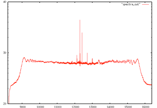
A power spectrum describes how the power of a signal or time series is distributed over different frequencies Because SAR uses a linear FM chirp, the power should always be distributed evenly in an image’s spectra. Because SAR data has distinctive range spectra, one method to check whether signals are valid SAR data is to plot the power spectra.
This was done early in data exploration, showing additional problems with the Seasat raw signal data. Rather than show the standard relatively flat peak, the Seasat spectra show tones that should not be present in raw data.
Seasat Range Spectrum: This plot shows the power spectrum of Seasat signal data plotted as a function of the range frequency bin. Although the DC Bias at bin zero is expected, the additional tones make this a “dirty” spectrum. The largest tone always appears at +/- fs/4, while the other spurious tones appear in a variety of frequency locations. [Figure created by Paul Rosen, JPL].
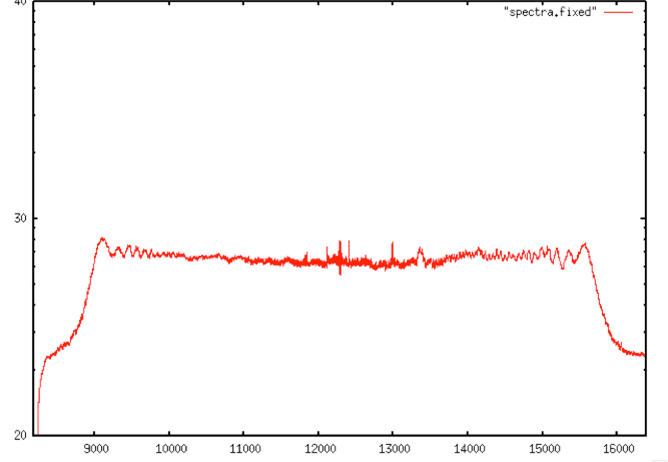
Fortunately, ROI has a built-in feature for the removal of specific frequencies that were inserted into the signal data for calibration purposes. These frequencies are called “caltones,” or calibration tones. The feature in ROI works as a notch filter, and ASF was able to modify it to remove up to 20 unwanted caltones. To determine the frequencies to remove, the steps outlined in the Spectral Filtering Algorithm were taken.
- Calculate the range power spectra
- Calculate the mean and standard deviation of the spectra
- Sort all spectral values that are greater than 1.5 standard deviations from the mean into descending order
- Cull the list to remove neighboring caltones: All tones within 6 bins of a tone previously in the list are removed. This ensures only a single frequency will be removed in given neighborhood of bins.
- Remove up to the top 20 values left in the list
Spectra Filtering Algorithm: All values greater than 1.5 standard deviations from the mean spectral value are gathered and sorted. Closely neighboring caltones are culled, creating the final list of caltones to be removed via notch filtering.
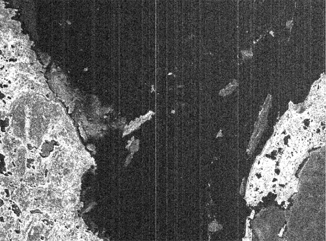
Once the power spectra have been filtered to remove these caltones, many artifacts are removed from the Seasat images.
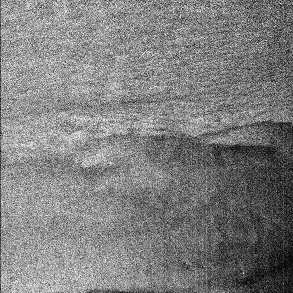
Unfiltered Spectra
Representation of the Filtered Spectra
Unfiltered Spectra
Filtered Spectra
Unfiltered Spectra
Filtered Spectra
8.5 Data Window Position Shifts
The time delay between transmitting a SAR pulse and receiving an echo is directly related to the altitude of the satellite at the time of imaging. Based upon changes in orbital altitude, this delay may change a handful of times in any given datatake. As the satellite altitude changes during an orbit, the change is quantified using the delay-to-digitization field. During focusing, the slant range to the first pixel is calculated using these quantified values.
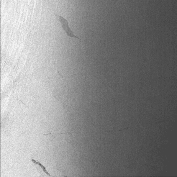
Prior to the application of the delay-to-digitization parameter in the ASF Seasat Processing System (ASPS), cross-track ghosting was readily observed in images that contained delay shifts. This was addressed using another one of ROI’s built in features – the data window position (DWP) file.
This file contains one entry for each delay-to-digitization shift found in a swath. Each such entry contains a <line, value> pair where line is the line number in the cleaned raw swath data to apply the shift and value is the amount of the shift. This DWP file is then passed to ROI where the DWP shift is implemented.
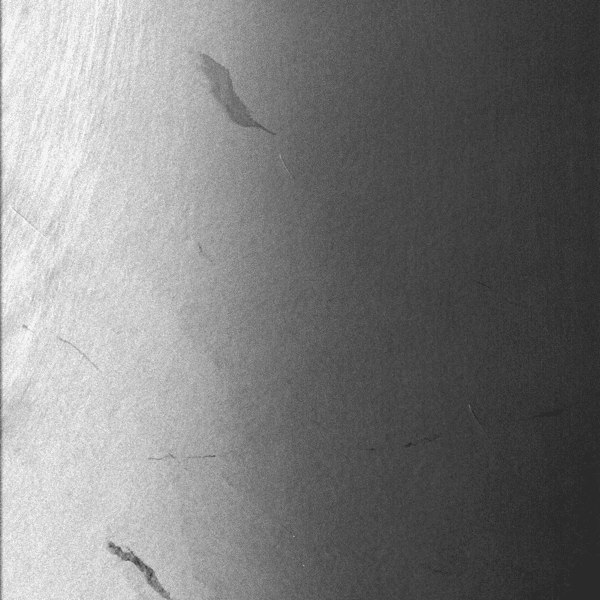
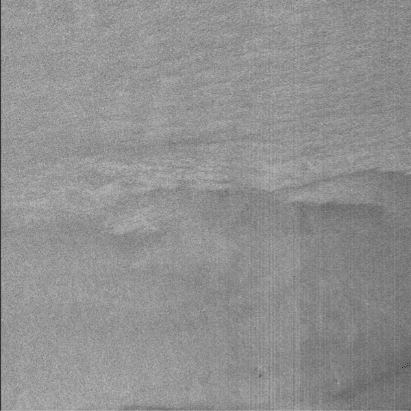
Cross-Track Ghosting

Ghosting Removed
Written by Tom Logan, July 2013
