
At this stage in the development of the ASF Seasat Processing System (ASPS):
- 1,346 cleaned raw signal swaths were created
- Repeat Orbit Interferometry (ROI) was modified to handle Seasat offset video format
- New state vectors were selected for use over two-line elements (TLE’s)
- Caltones were filtered from the range power spectra
- Data window position files were created
The remaining tasks before wholesale image creation could begin were (1) automated creation of the ROI input files with all fields properly filled and (2) implementation of a product framing scheme.
9.1 Creation of ROI Configuration Files
The program create_roi_in was developed for the purpose of gathering all of the information necessary to focus a particular piece of Seasat data into complex imagery.
create_roi_in:
- Using the .hdr file of metadata
- Determine exact start, center and end time of signal data section to be focused
- Find any changes in the delay-to-digitization in this section of signal data
- Create a DWP file if necessary, marking all shifts that occured
- Use the minimum DWP to calculate the slant range to first pixel
- Propagate the state vectors to the exact middle time of the scene and convert into ROI’s internal format for the spacecraft height, velocity and acceleration
- Estimate the Doppler centroid using filtering and regression to get a quadratic fit
- Calculate the range spectra, filter and get galtones to be removed
- Write all values to the .roi.in file
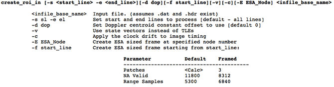
ROI Configuration File Creation Program: Many command line options are offered by create_roi_in, including the ability to process any amount of signal data or the exact amount of signal data needed to create a single 100-km2 image framed by European Space Agency (ESA) framing standards.
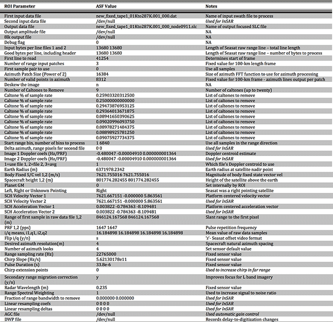
Modified ROI Configuration File: The ROI .in configuration file used to process image SS_00638_STD_F0911. ASF ROI configuration files allow for up to 67 lines of parameters to be passed. Note that ROI is the Repeat Orbit Interferometry correlator, and as such it is set up to process InSAR pairs of imagery. When utilized for processing single Seasat images, many ROI parameters are either not applicable or simply repeated (as in the case of input bytes per line, good bytes per line, spacecraft velocity, PRF, etc.). Most parameters are fixed based upon the sensor being focused. However, some parameters vary in each scene since they are either data dependent (i/q mean, caltones to remove, Doppler centroid) or platform-location specific (body fixed velocity, earth radius, spacecraft altitude, velocity and acceleration, range of first sample).
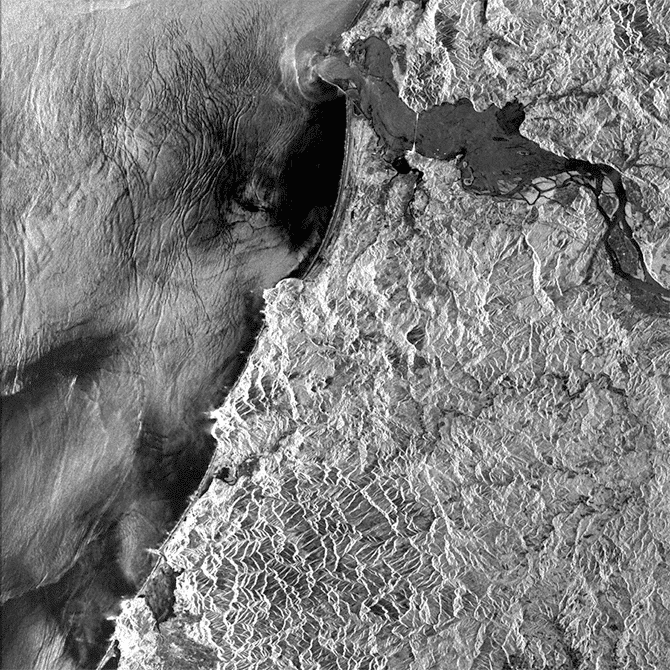
SS_00638_STD_F0911: Seasat image created using the parameters in the modified ROI configuration file.
9.2 Framing Data Products
ASF divides swaths of SAR data into individual frames that are bundled into products and made available for download. Seasat swaths are divided into 100-km2 scenes centered at European Space Agency (ESA) standard nodes. The naming convention for Seasat products is as follows:
SS_00000_STD_Fffff
Where 00000 is the five-digit orbit number of Seasat platform at time of imaging and ffff is the four-digit ESA node number signifying the center latitude of the product.
9.2.1 Modified ESA Frames – Product Length Determination
ASF elected to use the ESA node scheme as it is common to other products and understood by many SAR researchers. From “ESA EOHelp Frequently Asked Questions”:
The European Remote-Sensing Satellite (ERS) orbit is split into 7200 nodes and 400 are used to identify the SAR frames through the node closest to the frames’ center. Therefore, the identifiers of two adjacent frames differ by 18 nodes. The first frame starts at the equator and is identified by node 9, the last one by number 7191.
The frames between number 9 to 1791 and 5409 to 7191 are in the ascending part of the orbit.
A satellite orbit is split into two parts:
- the ascending pass
- the descending pass
The ERS-1 satellite has the following scheme:
Equator North Pole Equator South Pole Equator
9 1800 3609 5400 7191
|—ascending—|————–descending———–|—ascending—|
where the numbers are standard frame numbers
When the scheme above was implemented using frames centered 18 nodes apart, large gaps existed between the framed Seasat products. This can be explained as follows: splitting the earth up into 7,200 nodes means that each node is 0.05 degrees of latitude. If images are framed 18 nodes apart, then the centers are 18 * 0.05 degrees = 0.9 degrees of latitude apart. A degree of latitude varies from 110.6 km to 111.7 km from the equator to the North Pole. Therefore, 0.9 degrees of latitude varies from 99.54 km to 100.53 km from the equator to the North Pole.
It follows that even if the orbit of Seasat was directly north-south, little to no overlap could be expected for 100-km length scenes. However, Seasat had an orbital inclination of 108 degrees, a full 10 degrees further off vertical than ERS-1, the satellite for which ESA designed these nodes. Thus, Seasat covered considerably less latitude per 100 km of travel than the ERS satellites.
Nodes 0 – 1800: center latitude = node*.05
Nodes 1801 – 3600: center latitude = 180.0-(node*0.05)
ESA Frame Center Calculations: Nodes 0 – 1800 are ascending in the Northern hemisphere. Nodes 1801 – 3600 are descending the Northern hemisphere. Nodes 3601 – 7200 are located in the Southern Hemisphere, so they will never be used for the Seasat data collection.
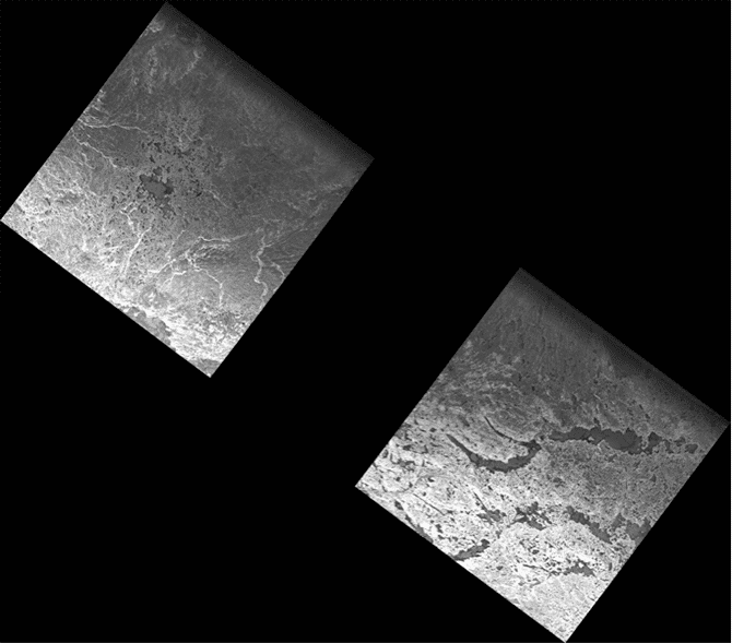
Using ESA Standard Frames: These images were framed using the standard ESA framing technique (frame 78 and 79) and then mosaicked to check for overlap. Since there is black between the images, the standard ESA framing schema is not valid for Seasat products.
Due to differences between the ERS-1 and Seasat orbits, a modified ESA scheme was implemented for Seasat products. At first, the number of nodes between framed centers was simply halved, i.e. products were created with centers only nine ESA nodes apart.
This scheme worked until the higher latitudes, where the satellite’s orbital path goes from ascending to descending. At this part of the orbit, the satellite actually stops ascending in latitude and starts descending. In this case, 100 km of satellite motion is considerably less than nine nodes of latitude change. Thus gaps once again existed between framed products.
Finally, then, the ASF Seasat SAR framing scheme allows a variable number of ESA nodes to pass between frames. Each frame is 100 km in length and centered at the ESA node that gives roughly 15 percent overlap with the adjacent frames. Thus all Seasat products are the same size but spaced variably along-track. Since Seasat only imaged in the Northern hemisphere, only ESA nodes 0 – 3600 are ever used.
Modified ESA Frames
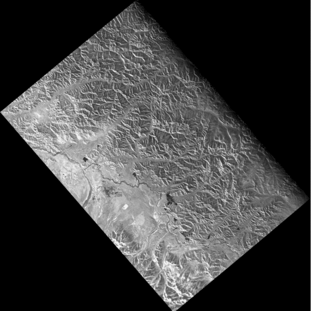
Modified ESA Frames: This mosaic shows two Seasat products created nine ESA nodes apart (1278 – 1287). In this case, the mosaic shows no gap exists between these framed products.
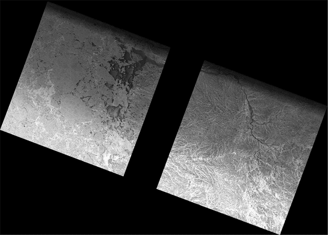
Modified ESA Frames: This mosaic also shows two Seasat products created nine ESA nodes apart (1467 – 1476). However, because these images are at a higher latitude, there is a gap between processed frames. The nine-nodes-between-centers method did not work properly for Seasat.
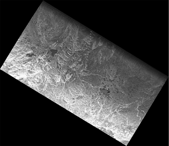
Framed Seasat Product Mosaic: Mosaic of two Seasat framed products showing how the modified schema with variable nodes between centers ensures overlap between framed products.
Aside: Example of Products Created from a Single Cleaned Swath – Processing cleaned swath file new_fixed_tape4_01Kto688K.001_000.dat resulted in the following list of products (ESA node numbers highlighted in blue):
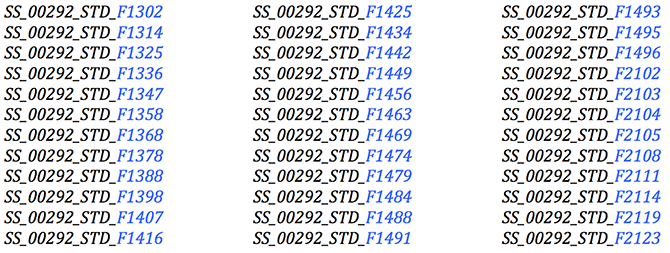
Note that orbit number 00292 goes from ascending (nodes 1302 – 1496) to descending (2102 – 2123). Note too how the ESA node numbers get closer together as the satellite approaches the northern tip of its orbit. The same applies in reverse on the descending part of the orbit: At first images are centered just one ESA node apart, but the number of nodes between frame centers grows as the satellite continues south.
9.2.2 Far Range Samples – Product Width Determination
SAR processing is performed on specifically sized pieces of signal data called patches. Patches are generally an even power of 2 in size to facilitate the FFTs that are used during focusing. Range patches are in the range direction; for Seasat only a single range patch of length 8192 is needed to process the entire range direction of 6,840 samples. Azimuth patches are in the azimuth direction. Azimuth patches can vary in length. For Seasat a length of 16,384 (16K) was used.
The SAR processing algorithm requires a certain amount of overhead per range patch and azimuth patch processed. This overhead is either the length of the azimuth reference function for the azimuth direction or the range reference function for the range direction. The length of these functions determines how many samples are combined to make a single return in the focused image. For Seasat, the range reference function is always 1,539 samples, while the azimuth reference function varies in length from around 5,500 to as much as 5,700.
Dealing with the overhead in the azimuth patches is straightforward. For each azimuth patch, process 16K lines of data and only keep 16K minus the patch overhead lines. Seasat processing only utilizes 8,312 lines per azimuth patch, well under the number of valid lines actually created.
The range reference function overhead is more difficult to deal with. All of the literature states that Seasat boasts a 100-km width swath. However, of the 6,840 range samples that can be created per line, only 5,301 samples are known to be valid (5,301 = 6,840 range samples minus the 1,539 overhead). When these samples are mapped from natural slant range spacing into 12.5-meter ground range spacing, 7,166 valid range samples are created. This means that the actual valid width of the Seasat swath is
7,166 samples * 12.5 meters/sample = 89,575 meters,
considerably less than the 100 km advertised.
Thus, it had to be determined if Seasat products should be 100 km 2, even if it meant keeping some partially valid samples in the far range, or should products be less than 100 km 2 , keeping only known valid pixels. The decision was made to create 100-km wide swaths even though this may introduce a few pixels in the far range that do not contain the contributions from a full 1,539 raw samples. As a result, users may notice slight darkening in the last 824 range samples in some images. This is intentionally done in order to create square Seasat products.
9.3 Data Quality Tool
Due to Doppler ambiguities that could not be automatically overcome, each Seasat product created at ASF is examined using a specially designed quality control tool. This QC tool allows each product to be visually inspected and accepted, reprocessed, or discarded. If a product is not focused, it is reprocessed at the next logical Doppler ambiguity. If a product contains less than 50% valid data it is discarded. Finally, if a product is accepted, an annotation file is made providing an indication of data quality issues observed in the product. Each of these remaining data quality issues will be discussed in “Quality Issues.”
9.4 Processing Results
Once the programs that create a single image product were developed and tested, they were all encapsulated in a main program referred to as create_base_images. Given an input cleaned swath file, create_base_images creates all framed products covered by a datatake. Each swath is run through this procedure in order to create the beta set of framed Seasat images and corresponding metadata.
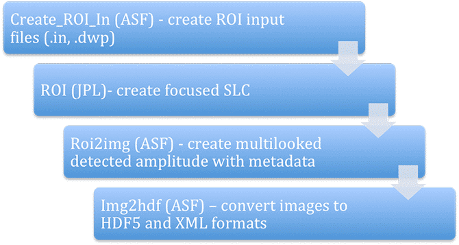
Single Image Processing Flow: In order to create an individual framed product, a cleaned swath file goes through (1) creation of the configuration file(s) for ROI, (2) focusing into SLC imagery using ROI, (3) creation of multilooked amplitude images, and (4) conversion of images into HDF5 with ISO compliant XML metadata.
Each of these images are visually examined using the ASF Seasat Quality Control Tool, which allows one of three actions to be taken:
- Images that show less than half a frame of valid SAR data are discarded.
- Images that are not properly focused are sent through a reprocessing step, which modifies the Doppler constant in order to determine a Doppler centroid that will focus the product.
- Images that are properly focused and contain more than 50 percent valid SAR data are added the to the ASF data pool. Each product also contains an annotation file to inform the end user of any quality issues encountered during the visual QC check.
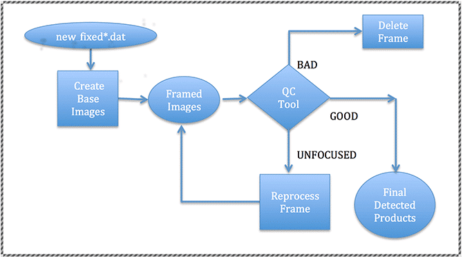
ASF Seasat Processing System (ASPS) V1.0: All cleaned decoded swaths were passed through the create_base_images procedure, which created the framed product files. Due to Doppler ambiguities and data quality issues, each product had to be examined using the QC Tool, which took one of three actions: (1) If the image is good, publish it; (2) If it is unfocused, reprocess it at a new Doppler; (3) If the image is not valid SAR data, delete the product.
Written by Tom Logan, July 2013
