

In order to create a synthetic aperture for a radar system, one must combine many returns over time. For Seasat, a typical azimuth reference function — the number of returns combined into a single focused range line — is 5,600 samples. Each of these samples is actually a range line of radar echoes from the ground. Properly combining all of these lines requires knowing precisely when a range line was received by the satellite.
In practice, SAR systems transmit pulses of energy equally spaced in time. This time is set by the pulse repetition frequency (PRF); for Seasat, 1,647 pulses are transmitted every second. Alternatively, it can be said a pulse is transmitted every 0.607165 milliseconds, an interval commonly referred to as the pulse repetition interval or PRI. Without this constant time between pulses, the SAR algorithm would break down and data would not be focused to imagery.
Many errors existed in the Seasat raw data decoded at ASF. As a result, multiple levels of filtering were required to deal with issues present in the raw telemetry data, particularly with time values. Only after this filtering were the raw SAR data processible to images.
4.1 Median Filtering and Linear Regression
The first attempt at cleaning the data involved a simple one-pass filter of the pertinent metadata parameters. The following seven parameters were median filtered to pull out the most commonly occurring value: station code, day of year, clock drift, delay to digitization, least significant digit of year, bits per sample and PRF rate code. A linear regression was used to clean the MSEC of Day metadata field. This logic is encapsulated in the program fix_headers, which is discussed in more detail in “Final Form of Fix_Headers.”
Implementing the median filter was straightforward:
- Read through the header file and maintain histograms of the relevant parameters.
- Use the local median value to replace the decoded value and create a cleaned header file. Here “local” refers to the 400 values preceding the value to be replaced.
This scheme works well for cleaning the constant and rarely changing fields. It also seems to work quite well for the smoothly changing clock drift field. At the end of this section are the examples from “Problems with Bit Fields,” along with the corresponding median-filtered versions of the same metadata parameters. In each case, the median filter created clean usable metadata files.
Performing the linear regression on the MSEC of Day field was also straightforward. Unfortunately, the results were far from expected or optimal. The sheer volume of bit errors combined with discontinuities and timing dropouts made the line slopes and offsets highly variable inside a single swath. These issues will be examined in the next section.
Table of Filtered Parameters
| Parameter | Filter Applied | Value |
|---|---|---|
| station_code | Median | Constant per datatake |
| day_of_year | Median | Varies |
| clock_drift | Median | Varies |
| delay_to_digitization | Median | Varies |
| least_significant_digit_of_year | Median | 8 |
| bit_per_sample | Median | 5 |
| prf_rate_code | Median | 4 |
| msec_of_day | Linear Regression | Varies |
Data Cleaning Examples
Station Code
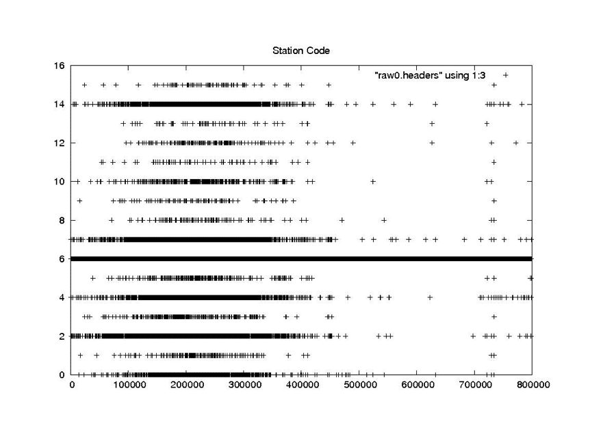
RAW
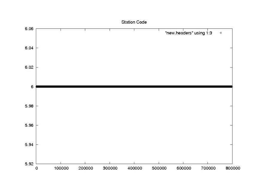
NEW
Day of Year
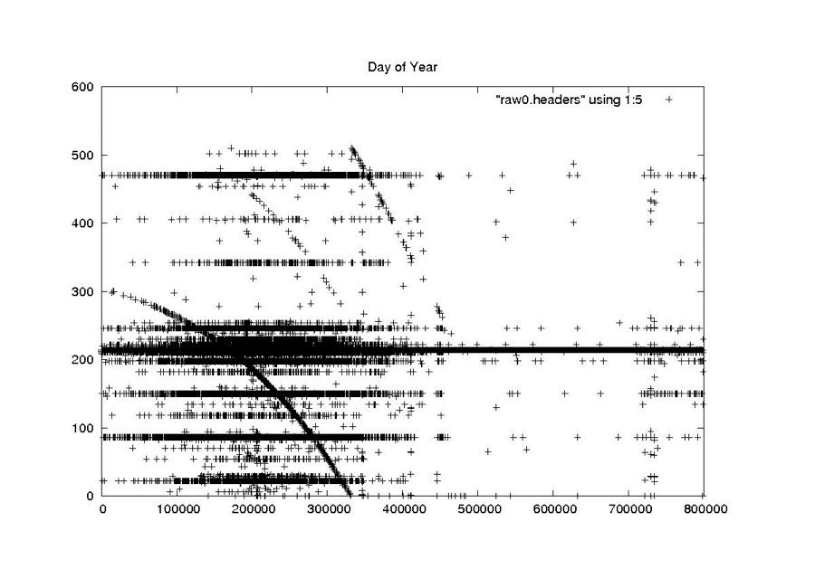
RAW
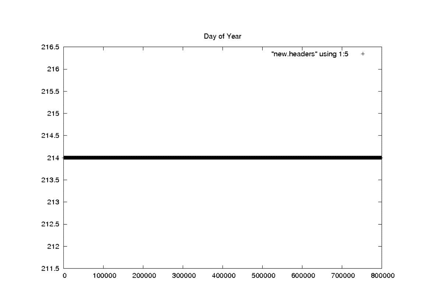
NEW
Last Digit of the Year
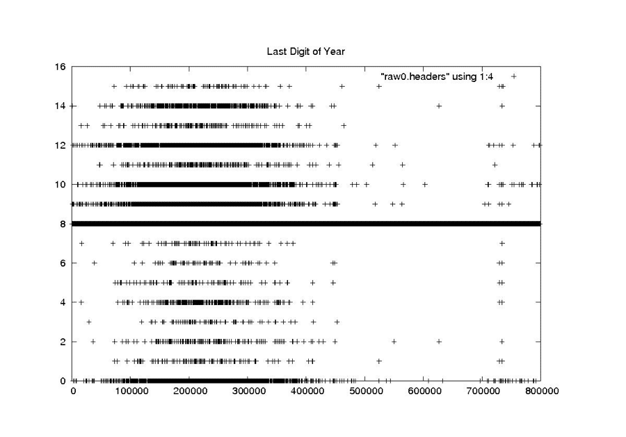
RAW
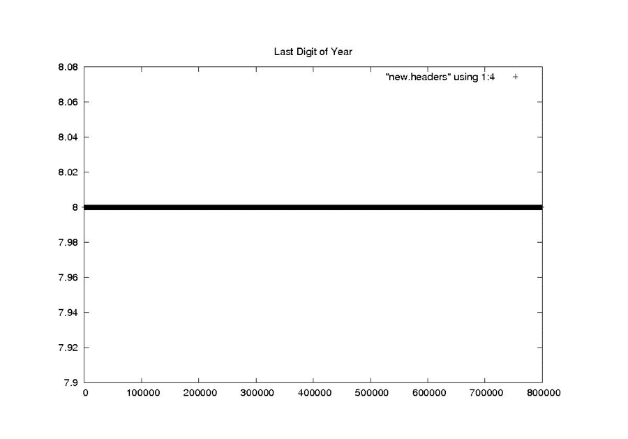
NEW
Clock Drift
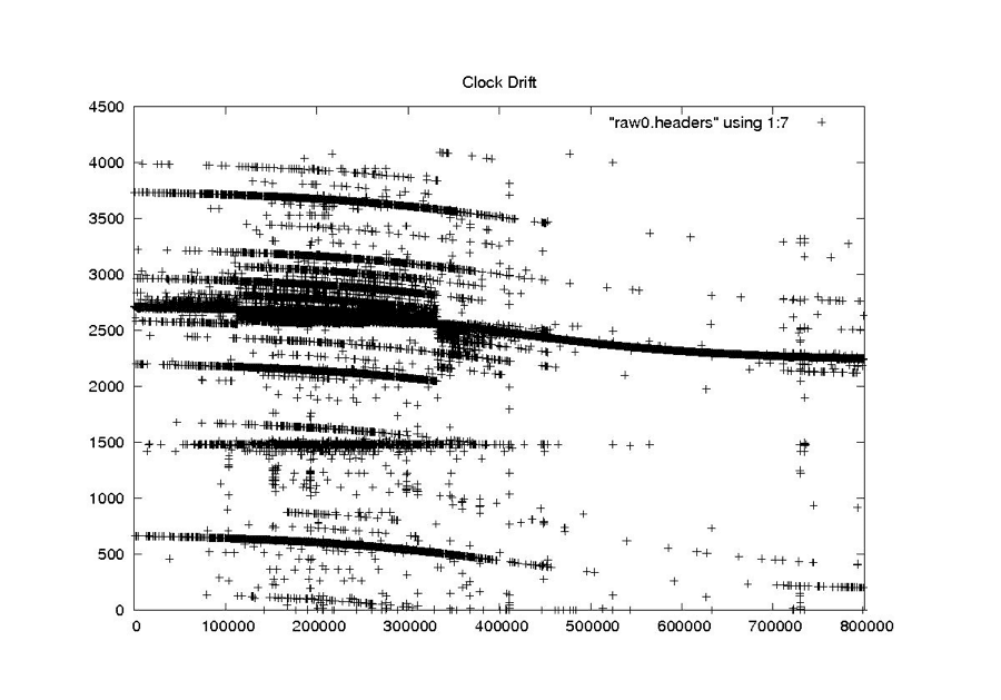
RAW
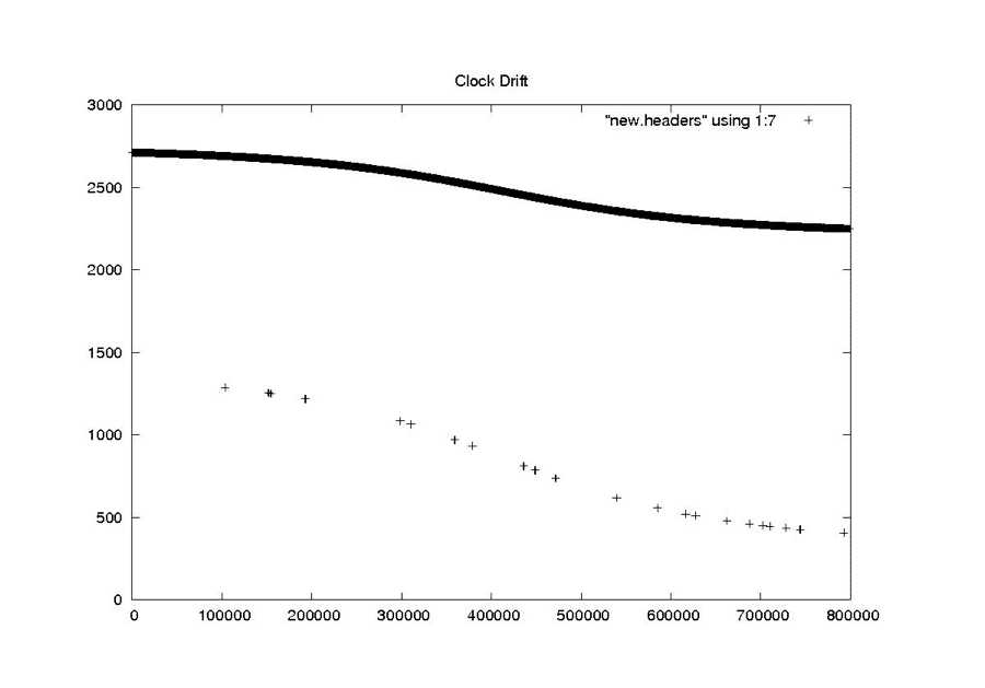
NEW
Bits Per Sample
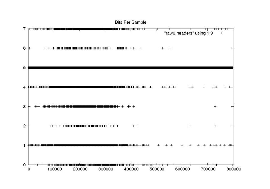
RAW

NEW
PRF Rate Code
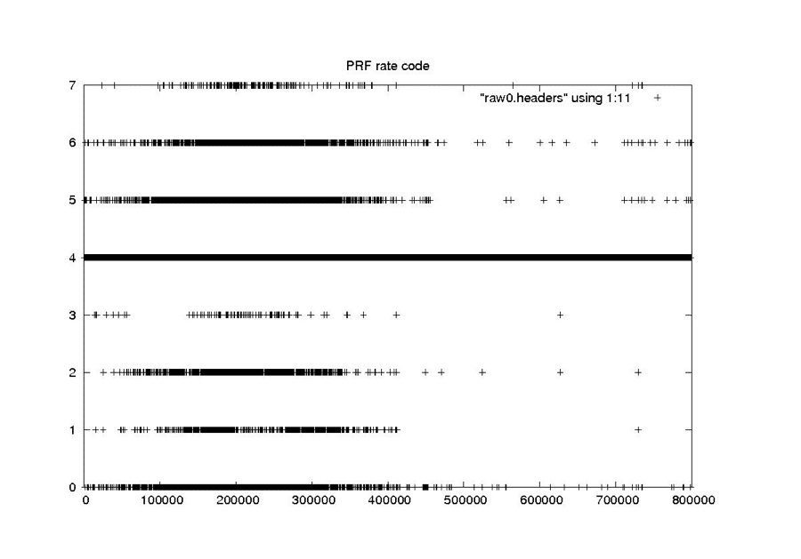
RAW
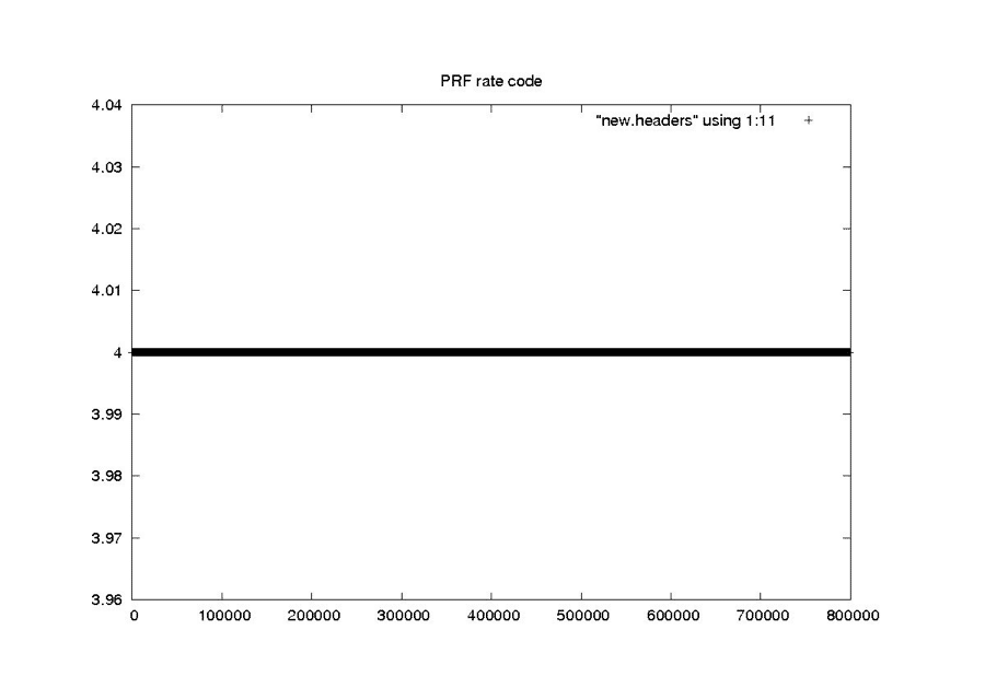
NEW
Delay to Digitzation
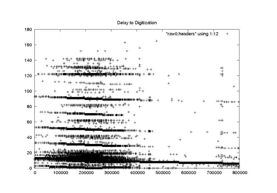
RAW
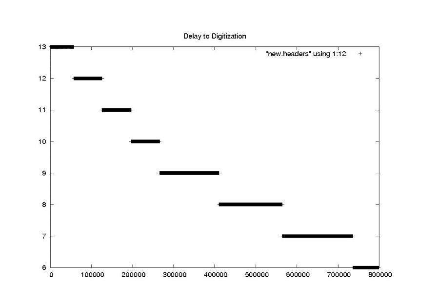
NEW
4.2 Time Cleaning
Creating a SAR image requires combining many radar returns over time. This requires that very accurate times are known for every SAR sample recorded. In the decoded Seasat data, the sheer volume of bit errors, combined with discontinuities and timing dropouts, resulted in highly variable times inside a single swath.
4.2.1 Restricting the Time Slope
One of the big problems with applying a simple linear regression to the Seasat timing information was that the local slope often changed drastically from one section of a file to another based upon bit errors, stair steps and discontinuities. Since a pulse is transmitted every 0.607165 milliseconds, it seemed that the easiest way to clean all of the MSEC times would be to simply find the fixed offset for a given swath file and then apply the known time slope to generate new time values for a cleaned header file.
This restricted slope regression was implemented when it became obvious that a simple linear regression was failing. By restricting the time slope of a file to be near the 0.607-msec/line known value, it was assumed that timing issues other than discontinuities could be removed. The discontinuities would still have to be found and fixed separately in order for the SAR focusing algorithm to work properly. Otherwise, the precise time of each line would not be known.
4.2.2 Removing Bit Errors from Times
fix_time
- Crude time filtering, trying to fix all values that are > 513 from local linear trend:
- Bit fixes – replace values powers of 2 from trend
- Fill fixes – fill gaps in constant consecutive values
- Linear fixes – replace values with linear trend
- Reads and writes a file of headers
Even with linear regressions and time slope limitations, times still were not being brought into reasonable ranges. Too many values were in error in some files, and a suitable linear trend could not be obtained. So, another layer of time cleaning was added as a pre-filter to the final linear regression done in fix_headers. The program fix_time was initially created just to look for bit errors, but was later expanded to incorporate each of three different filters at the gross level (i.e. only values > 513 from a local linear trend are changed):
- If the value is an exact power of 2 off from the local linear trend, then add that power of 2 into the value. This fix attempts to first change values that are wrong simply because of bit errors. The idea is that this is a common known error type and should be assumed as the first cause.
- Else if the value is between two values that are the same, make it the same as its neighbors. This fix takes advantage of the stair steps found in the timing fields. It was only added in conjunction with the fix_stairs program discussed below. The idea is to take advantage of the fact that the stair steps are easily corrected using the known satellite PRI.
- Else just replace the value with the local linear trend. At this point, it is better to bring the points close to the line than to leave them with very large errors.
4.2.3 Removing Stair Steps from Times
fix_stairs
- Fix for sticky time field – Turns “stairs” into “lines” by replacing repeated time values with linear approximation for better linear trend
- Reads and writes a file of headers
For yet another pre-filter, it was determined that the stair steps time anomaly should be removed before fitting points to a final linear trend. This task is relatively straightforward: If several time values in a row are the same, replace them with values that fit the known time slope of the satellite. The program fix_stairs was developed to deal with this problem.
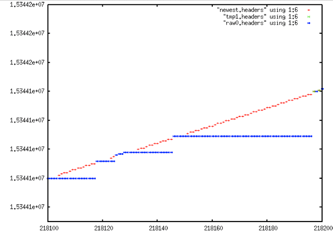
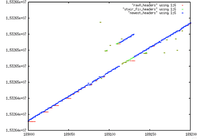
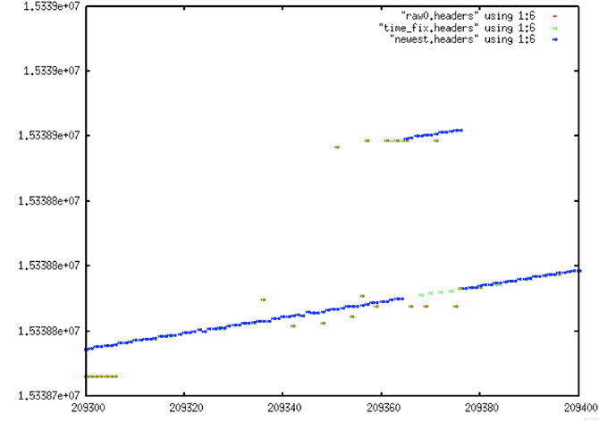
Extreme Stair Step: raw0.headers (blue) are the original unfiltered MSEC time values; newest.headers (red) shows the result of fixing the “stairs” that result from the sticky clock, presumably an artifact of the Seasat hardware, not the result of bit rot, transcription or other errors
4.2.4 Final Form of fix_headers
fix_headers
- Miscellaneous header cleaning using median filters:
- Station Code
- Least Significant Digit of Year
- Day of Year
- Clock Drift
- Bits Per Sample
- PRF Rate Code
- Delay to Digitization
- Time Discontinuity Location and Additional Filtering
- Replace all values > 2 from linear trend with linear trend
- Locates discontinuities in time, making an annotated file for later use.
- 5 bad values with same offset from trend identity a discontinuity
- +1 discontinuity is forward in time and can be fixed
- if > 4000, too large – cannot be fixed
- otherwise, slide time to fit discontinuity
- if offset > 5 time values, save this discontinuity in a file
- -1 discontinuity is backwards in time and cannot be fixed
- Reads and writes a file of headers
Although it started out as the main cleaning program, fix_headers is currently the final link in the cleaning process. Metadata going through fix_headers has already been partially fixed by reducing bit errors, removing stair steps, and bringing all other values that show very large offsets into a rough linear fit. So in addition to performing median filtering on important metadata fields (see section 4.1), this program performs the final linear fit on the time data.
Initially, a regression is performed on the first window of 400 points and used to fix the first 200 time values of that window. Any values that are more than 5 msec from their predecessors are replaced by the linear fit. After this, a new fit is calculated every window/2 samples, but never within 100 samples of an actual discontinuity. The final task for fix_headers was to locate the rough locations of all real discontinuities that occur in the files. At least, it was designed to only find real discontinuities – those being the final problem hindering the placement of reasonable linear times in the swath files.
Identifying discontinuities was challenging. Much trial and error resulted in a code that worked for nearly all cases and was able to be configured to work for the other cases as well. The basic idea is that if a gap is found in the data, and if after the gap no other gaps occur within 5 values, then it is possible that a discontinuity exists. If so, the program determines the number of lines that would have to be missing to create such a gap and records the location and size in an external discontinuity file. Note that only forward discontinuities can be fixed in this manner and only discontinuities less than a certain size. In practice, the procedure attempts to locate gaps of up to 4,000 lines, discarding any datasets that show gaps larger than this.
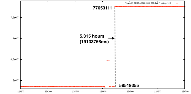
Extreme Discontinuity: This decoded signal data shows a 5.3-hour gap in time. This cannot be fixed.
In the end, all of the gaps in the data were identified, and, there is high confidence that any such discontinuities found are real and not just the result of bit errors or other problems. Unfortunately, this method was not able to pinpoint the start of problems, only that they existed, as shown in the following set of graphs.
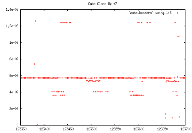
Decoded Signal Data with No Y-range Clipping
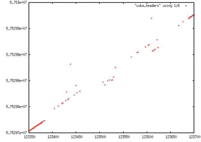
Decoded Signal Data with Y-range Clipping
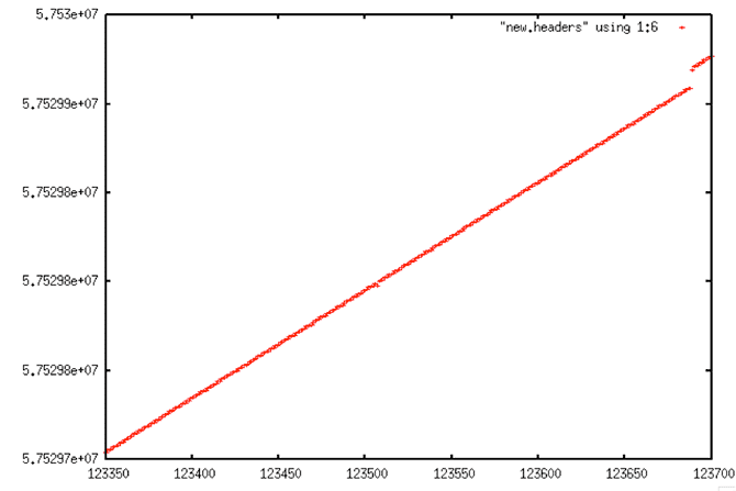
Linear Trend of Decoded Signal Data
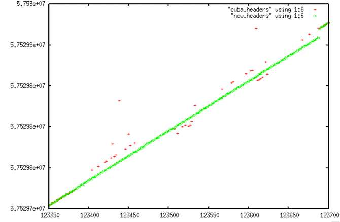
Comparison of Decoded Signal Data and Linear Fit
False Discontinuity #1
False Discontinuity #2
4.2.5 Removing Discontinuities
dis_search
- fix all time discontinuities in the raw swath files
- for each entry in previously generated discontinuity file:
- search backwards from discontinuity looking for points that don’t fit new trend line
- when 20 consecutive values that are ont within 1.5 of new line are found, you have found start of discontinuity
- For length of discontinuity
- Repeat header line in .hdr file (fixing the time only)
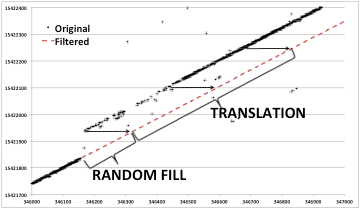
- Fill .dat file with random values
- Reads discontinuity file, original .dat and .hdr file, and cleaned .hdr file. Creates final cleaned .dat and .hdr file ready for processing
- for each entry in previously generated discontinuity file:
The first task in removing the discontinuities is locating them. The rough area of each real discontinuity can be found using the fix_headers code as described in the previous section.
Finding the exact start and length of each discontinuity still remains to be done. This search and the act of filling each gap thus discovered is performed by the program dis_search. The discontinuity search is performed backward, with 3000 lines after each discontinuity area being cached and then searched for a jump down in the time value to the previous line. These locations were marked as the actual start of the discontinuity. The gap in the raw data between the time before the discontinuity and the time after must then be filled in. Random values were used for fill, these being the best way to not impact the usefulness of the real SAR data.
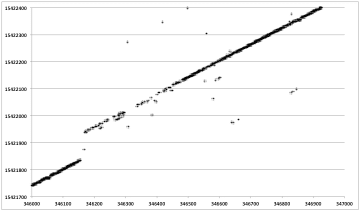
Discontinuity Fills: Each plot shows range line number versus MSEC metadata value. Original decoded metadata (left) is spotty and contains an obvious time discontinuity. After the discontinuity is found and corrected, linear time is restored (right).
